Z-Stats / Basic Statistics
Z-8: Two-Sample and Directional Hypothesis Testing
This lesson describes some refinements to the hypothesis testing approach that was introduced in the previous lesson. The truth of the matter is that the previous lesson was somewhat oversimplified in order to focus on the concept and general steps in the hypothesis testing procedure. With that background, we can now get into some of the finer points of hypothesis testing.
EdD, Assistant Professor
Clinical Laboratory Science Program, University of Louisville
Louisville, Kentucky
October 1999
- Two-sample case
- Directional vs. non-directional testing
- Critical t-values for one-tailed and two-tailed tests
- About the Author
This lesson describes some refinements to the hypothesis testing approach that was introduced in the previous lesson. The truth of the matter is that the previous lesson was somewhat oversimplified in order to focus on the concept and general steps in the hypothesis testing procedure. With that background, we can now get into some of the finer points of hypothesis testing.
Two sample case
The "two sample case" is a special case in which the difference between two sample means is examined. This sounds like what we did in the last lesson, but we actually looked at the difference between an observed or sample group mean and a control group mean, which was treated as if it were a population mean (rather than an observed or sample mean). There are some fine points that need to be considered about the calculations and the procedure.
Refinements in calculations
Mathematically, there are some differences in the formula that should be used. Recall the form of the equation for calculating a t-value:

where Xbar is the mean of the experimental group, and µ is a population parameter or the mean of the population. In the last lesson, we substituted the control group mean XbarB for µ. However, the control group was actually a sample from the population of all such mice (in this example) and following suit, the experimental group was also just a sample from its population. Phrasing the situation this way, there are now two sets of differences that must be considered: the difference between sample means or XbarA-XbarB and the difference between population means from which these samples came or µA-µB. Those expressions should be substituted into the tcalc formula to give the proper mathematical form:

- In this new equation, the difference between means (Xbar A - XbarB) is called bias and is important in determining test accuracy, so even though this discussion is getting more complicated, the statistic that we are deriving is very important.
- The new error term is called the pooled estimate of the population variance and is derived from the difference scores from the two samples, as follows:
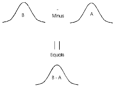
 It just so happens that the distribution of the differences between two means approximates a normal distribution given a certain N. See Figure 8-1.
- In the expression for the pooled variance, the XAs represent the individual values or scores for test A. The mean of the sample from which a value was taken (XbarA) is subtracted from the XAs yielding a difference score. The sum (
 ) of the difference values for the entire sample of A values is squared. The same is done with sample B. The difference is averaged over N's. The minus 2 in the denominator represents the fact that 2 df's have been lost, one for each group.
 - Since the expression
 (XAs-XbarA) squared is the sum of the squared differences (SS) for A, the formula can be changed to:

- When the square root is taken, the result is called the standard deviation of the difference between means, SDd, which is shown by the formula:

- The proper equation for calculating the t-value for the two-sample case then becomes:

Refinements in procedure
Remember the steps for testing a hypothesis are: (1) State the hypotheses; (2) Set the criterion for rejection of Ho; (3) Compute the test statistic; (4) Decide about Ho.
- The null hypothesis can be stated as: Ho: µA = µB or µA - µB = 0. But it may be more revealing to say Ho: (XbarA-XbarB) - (µA - µB) = 0. The difference between the sample means minus the difference between the population means equals zero.
- The alternative hypothesis can be stated as: Ha: µA is not equal to µB or Ha: (XbarA-XbarB) - (µA - µB) is not equal to 0, i.e., the means of the two groups are not equal.
- The criteria for rejection or the alpha level is 0.05.
4
- The test statistic is computed as:
- Since it is hypothesized that the two methods are comparable and the difference between the means of the two populations is zero (µA - µB = 0), the calculation can be simplified as follows:

- If this tcalc is greater than 1.96 then the null hypothesis of no difference can be overturned (p0.05).
- Even though we have used several different mathematical formulae, the interpretations are the same as before.
Directional hypothesis testing vs non-directional testing
Remember the example of testing the effect of antibiotics on mice in Lesson 7. The point of the study was to find out if the mice who were treated with the antibiotic would outlive those who were not treated (i.e., the control group). Are you surprised that the researcher did not hypothesize that the control group might outlive the treatment group? Would it make any difference in how the hypothesis testing were carried out? These questions raise the issue of directional testing, or one-tailed vs two-tailed tests.
A two-tailed test for our mice
 Now don't get confused - we're not testing to see if our mice have two tails! We're testing to see if the mean of the sample group is either less than or greater than the mean of the control group, which - in statistical terms - is considered to be a two-direction or two-tailed test. Remember that the hypotheses were Ho:XbarA = XbarB and Ha: XbarA is not equal to XbarB. In this alternate hypothesis, all that has been said is that the two means are not the same, which would be true (a) if the mean of the sample group is higher than that of the control group or (b) if the mean of the sample group is lower than that of the control group. There is nothing in the phrasing of the hypothesis that stipulates the group A animals (treated) must actually have longer life spans as compared to the group B animals.
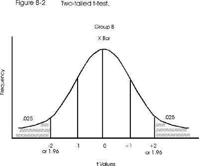
The issue of two-side vs one-side tests becomes important when selecting the critical t-value. In the earlier discussion of this example, the alpha level was set to 0.05, but that 0.05 was actually divided equally between the left and right tails of the distribution curve. The condition being tested is that group A has a "different" life span as compared to group B, which represents a two-tailed test as illustrated in Figure 8-2.
A one-tailed test for our mice
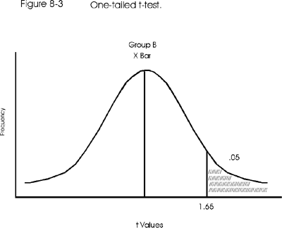
 If the conclusion were to support the claim that the antibiotic prolonged group A life spans, then the researchers should use a directional alternate hypothesis, such as Ha: XbarA > XbarB. Here group A's life span is hypothesized to be greater (longer) than group B's (the control group). In this case, an alpha level of 0.05 implies that all 0.05 would have to appear in the right or high tail of the curve, which then is a one-tailed or directional test, as shown in Figure 8-3. This figure shows that the critical t-value will actually be smaller for the one-tail test, that is, +1.65 instead of 1.96 or 2.00 from the two-tail test. This happens because 95% of the area under the curve begins to accumulate from the left-most side of the curve (including that tail) and includes less of the right side of the curve. The result is that tcalc can be smaller (1.65 instead of 1.96) and still cause Ho to be rejected.
Critical t-values for one-tailed and two tailed tests
This can be confusing and it should be helpful to think about having one or two gates on the curve. For example, for an alpha level of 0.05 and a two-tail test, there are two gates - one at -1.96 and one at +1.96. If you "walk" out of either of those gates, then you have demonstrated significance at p=0.05 or less. For a one-tail test, there is only one gate at +1.65. If you "walk" out of this gate, you have demonstrated significance at p=0.05 or less.
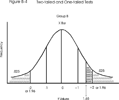
 The t-table provides for one-tailed versus two-tailed tests listing separate tcrit. As in all t-tests, in order to reject Ho and accept Ha (that group A lives longer than group B), the calculated t would have to be greater than the tcrit found in the table. But with the one-tail test the tcrit is 1.65 instead of 1.96, so tcalc may be smaller as well when rejecting Ho. It is actually easier to reject Ho using a one-tailed t-test. Figure 8-4 superimposes the two graphs in order to demonstrate the last statement.
For example, given a tabled t value (tcrit) of 1.96 at 0.05 significance for a 2-tailed t-test and a tcalc of 1.90, the Ho cannot be rejected. We are 0.06 away from walking out the gate. Using the one-tail test, this same value for tcalc exceeds the 1.65 tcrit for 0.05 alpha level, so the Ho can be rejected. We have walked out the gate and are standing a distance of 0.25 outside. So tcrit for a one-tail test is less than that for a two-tail test, at comparable alpha levels. That is, it takes less of a calculated t to overturn Ho. This relationship is shown in Figure 8-4. There is another more interesting point to be made. The figure actually shows that if you used a tcrit of 1.96 on a one-tailed test, the alpha level would actually drop to half of what it was before, from 0.05 to 0.025!
To reiterate, if you are standing right at the gate (1.96) for a two-tail test, then you have just barely met the p=0.05 requirement. However, if you are standing at the 1.96 point when running a one-tail test, then you have already exceeded the 1.65 gate and the probability must be even more significant, say p=0.025. It's important to find the critical t-value that is correct for the intended directional nature of the test.
About the author: Madelon F. Zady
Madelon F. Zady is an Assistant Professor at the University of Louisville, School of Allied Health Sciences Clinical Laboratory Science program and has over 30 years experience in teaching. She holds BS, MAT and EdD degrees from the University of Louisville, has taken other advanced course work from the School of Medicine and School of Education, and also advanced courses in statistics. She is a registered MT(ASCP) and a credentialed CLS(NCA) and has worked part-time as a bench technologist for 14 years. She is a member of the: American Society for Clinical Laboratory Science, Kentucky State Society for Clinical Laboratory Science, American Educational Research Association, and the National Science Teachers Association. Her teaching areas are clinical chemistry and statistics. Her research areas are metacognition and learning theory.
