Basic Method Validation

Determining Limit of Detection can be a challenge. Here's Part One of a discussion on how to do it.

Probit Analysis 1: Practical Application to Determine Limit of Detection

James O. Westgard, Sten A. Westgard
August 2020

In evaluating the performance of qualitative tests that provide binary results, accuracy is assessed by a clinical agreement experiment that compares results from the new test to an established or approved comparative test, or alternatively by comparison to the clinical diagnosis (disease, no disease). Much has been written about the clinical agreement study and the data analysis to determine clinical sensitivity (Se), clinical specificity (Sp), and the predictive value of a test for the expected prevalence of disease in the population of interest. CLSI provides a consensus document (EP12-A2) that describes good laboratory practices for performing a clinical agreement study, including detailed directions for analyzing the experimental data [1].

EP12 also describes a replication experiment for characterizing the “imprecision curve” or “imprecision interval” that describes the uncertainty of classification for binary results. Classification is based on a cutoff (CO) that might be set at the limit of detection (LoD) to maximize Se or somewhat higher to maximize Sp, with possible loss of Se. Given that Se and Sp depend on LoD or CO, the validation of LoD or CO is critical for characterizing the performance of a qualitative test.

See even more stories about COVID-19 Laboratory Challenges...

In this age of COVID-19, with the rapid introduction of many new molecular tests for diagnosis and antibody tests for surveillance, the FDA granted Emergency Use Authorization (EUA) based on minimal validation data by manufacturers to prove their performance claims. That leaves laboratories with increased responsibilities for assuring the quality of these new tests and methods by validating accuracy from their own clinical agreement studies and precision from their own estimation of LoD or CO.

There is much discussion and guidance in the literature for assessing accuracy from clinical agreement studies, but less about assessing precision by characterizing the imprecision curve and/or cutoff interval. CLSI does address both in the EP12-A2 document and also provides another consensus document (EP17-A2) on determination of limits of detection [2].

Estimation of LoD

For a quantitative test, the limit of detection (LoD) can be determined by analyzing two samples in replicate. First, a blank sample is analyzed with 20 replicates and the Limit of the Blank (LoB) calculated from the mean and SD, as follows:

LoB = Mean_blk + 1.65 SD_blk

Next, 20 replicates are determined for a low positive sample, the mean_pos and SD_pos calculated, and the Limit of Detection (LoD) calculated, as follows:

LoD = LoB + 1.65 SD_pos

This methodology assumes a continuous measurement scale, which may or may not be available for qualitative tests. For ELISA immunoassays, there is often an internal continuous response (ICR) that is converted to a binary result by comparison of the response signal to the cutoff. For simple linear flow devices, such a response is usually not available, in which case a different experimental methodology is required. Replicate measurements are made for three or more solutions near the cutoff. The concentration at the cutoff is described as C50 where half of the measurements are expected to be positive and half negative. At the low side of the cutoff, a replication experiment for a concentration of C5 would result in 1 positive out of 20 replicates (1/20=5%). At the high side of the cutoff, a concentration of C95 should yield 19 positives out of 20 (19/20=95%).

The figure below illustrates a test with a continuous response (top half) compared to a test with only a binary output (bottom half) for the condition where the LoD is equal to the CO.

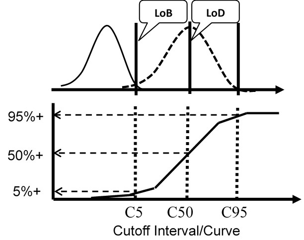
For the test with a continuous response, the means and SDs are determined for a blank sample and a low positive sample and the LoD calculated from the equations above. For the test with binary results, the positive proportions of replicate measurements at concentrations of C5, C50, and C95 are determined to characterize the cumulative probability distribution.

The important idea here is that the cumulative probability distribution provides an alternate way for evaluating the uncertainty of the test from an experimentally determined imprecision curve. Instead of analyzing replicates to determine a mean and SD, replicates are analyzed to determine the positive proportion, positivity rate, detection rate, or “hit rate.” Those results then characterize the cumulative distribution that describes the variation or uncertainty in the classification of patients at the cutoff limit.

For Nucleic Acid Amplification Tests (NAAT), the traditional approach requiring measurement of the blank cannot be applied because there is no variation for a blank solution, only a zero result is obtained. Therefore, instead of estimating C50 of the imprecision curve, the common approach is to estimate C95 either from hit rate directly or from probit regression of the observed hit rates versus concentrations of test solutions that characterize the imprecision interval.

Probit analysis

This type of statistical analysis is new to many clinical laboratory scientists, but it has been used in agriculture for biologic assays since the 1940s for characterizing dose response curves. The classic technique is found in the book authored by D. J. Finney and published in 1947 [3, Probit Analysis – A statistical treatment of the sigmoid responses curve]. The approach was used for toxicology applications, e.g., to characterize the dose of chemicals necessary to kill insects. The experimental approach determines the “kill rates” (proportion of insects killed) by increasing doses of insecticides, then converts those proportions to “probits”, which are “probability units” related to the number of standard deviations in a normal distribution. The model is the S-shaped or sigmoid curve that corresponds to the cumulative probability for a normal distribution, as shown below, where probability or hit rate (today’s common terminology related to kill rate) is plotted vs a standardized normal deviate, SD.

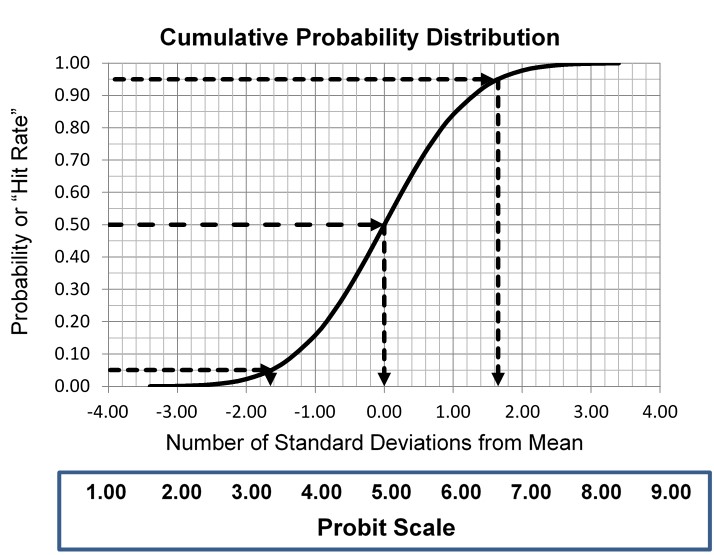
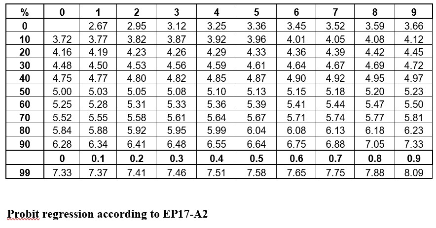
 The idea is to convert proportions to probability units on the SD scale. To keep the probability units positive for mathematic convenience, the probit scale adds a value of 5 to the number of standard deviations. A probit of 5.0 corresponds to the midpoint or concentration of C50, 6.64 corresponds to C95, and 3.36 to C5. The conversion of proportions or hit rates to probits can be carried out using the tables provided by Finney (see below), or by an Excel function 5+NORMSINV(P), where P is the proportion or hit rate that has been calculated from the raw data.

Probit regression according to EP17-A2

The purpose of linearizing the S-shaped imprecision curve is to enable fitting a model, in this case a straight line, to the data showing probability vs concentration. It is simple enough to estimate the LoD directly from the hit rate if test solutions can be pinpointed on C95. However, given that the LoD isn’t known exactly, a more practical approach is to analyze a series of concentrations, fit a line to those data points, then calculate/predict the C95 concentration.

A descriptive example is provided in EP17-A2 [2, page 23], as shown below.

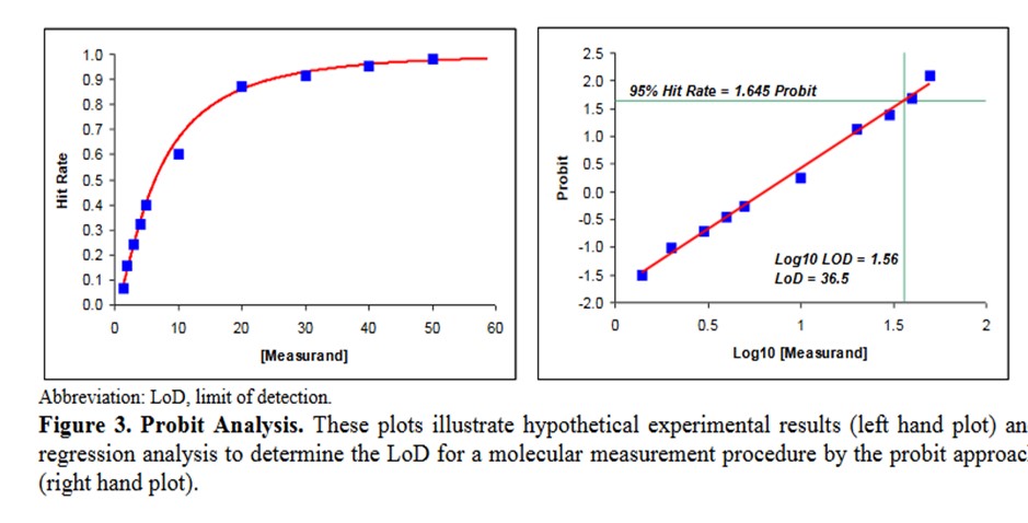
Some comments on this example:

• This data describes an NAAT test where the bottom of the S-shaped curve is not represented because there is no variation for a blank or zero concentration.
• The probit used is simply the number of SD, both plus and minus, rather than the probit scale from Finney where all values are positive.
• The probit regression uses a log transformation of the concentration for the x-axis. This is a common transformation for evaluating dose-response curves and is generally used when estimating LoD for NAATs.
• The estimate of the C95 concentration for LoD is obtained from first predicting the log10 value of 1.56, which must then be transformed back to a concentration of 36.5.

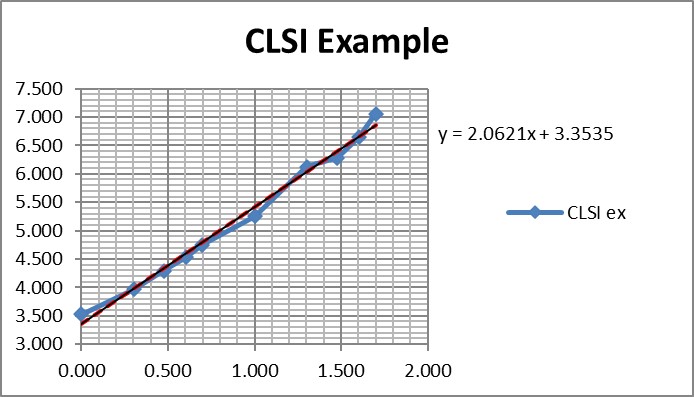
Reconstructed Example

Shown below is a data table that attempts to reconstruct the EP17-A2 example. The concentrations are likely correct as they proceed in a logical and orderly fashion. The total number of replicates (Ntotal) was set to 100 for ease of calculation, allowing the number of positives (Npos) to be approximated by the proportion read from the plot of hit rate vs concentration. The Probit was calculated by the Excel function [5+NORMSINV(P)], where P was the cell number in the proportion column.

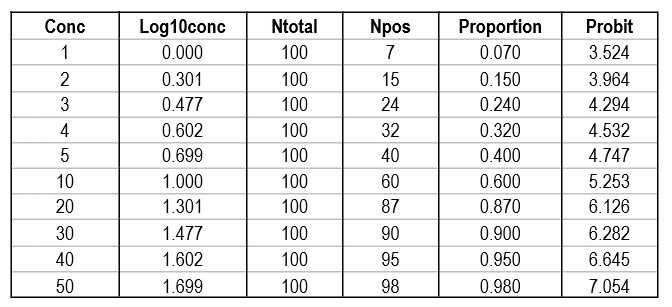
Regression gave a slope of 2.062 and a y-intercept of 3.353. To calculate C95, a probit value of 6.64 was used (1.64 for 95% limit, +5 for probit scale), which gave an estimate of 39.2 for the LoD. That compares with 36.5 as the CLSI answer, which is reasonably close given that all the data points were reconstructed by estimates from a graph.

It is useful to see the graph in order to judge the reliability of the data for fitting the regression model [see below]. In this example, there are 10 data points to provide a reliable regression, but in practice there often are fewer. EP17-A2 recommends a minimum of 3 data points between C10 and C90, one close to C95, and another outside of C5 the C95 range. The limited number of data points is one of the real limitations in published studies. Another is the lack of graphical evidence that the regression model provides a good fit to the data.

 A Real-World Example

The performance of the Cepheid Xpert Xpress SARS-CoV-2 test was assessed in a multicenter study by 8 laboratories, 5 in the US, 1 in France, 1 in Italy, and 1 in the United Kingdom [4].

The virus stock 9.75 x 10⁵ plaque forming units (PFU/mL) was obtained from the University of Texas Medical Branch Arbovirus Reference Collection, Galveston, TX. The limit of detection was determined by diluting the SARS-CoV-2 virus into negative NPS clinical matrix to 7 different levels near the estimated LoD ranging from 0.0200 to 0.0001 PFU/mL. A minimum of 22 replicates were tested at each level, including negatives. Probit regression analysis was utilized to estimate the LoD. The LoD was verified by spiking the SARS-CoV-2 virus into negative NPS clinical matris to the estimated LoD value previously determined by Probit regression analysis. A minimum of 22 replicates were tested for LoD verification… The positivity rate observed was ≥ 95% at a SARS-CoV-2 concentration of 0.005 PFU/mL. Of the 22 positive replicates tested at the LoD level of 0.01 PFU/mL, 22/22 (100%) reported a positive result.

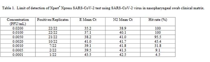
This is a good study that provides 5 data points in the useful probit range. According to the results, probit regression gave an estimate of 0.005 PFU/mL for the LoD, which was verified by a hit rate of 100% for the next highest concentration of 0.01 PFU/mL. Shown below is the probit graph.

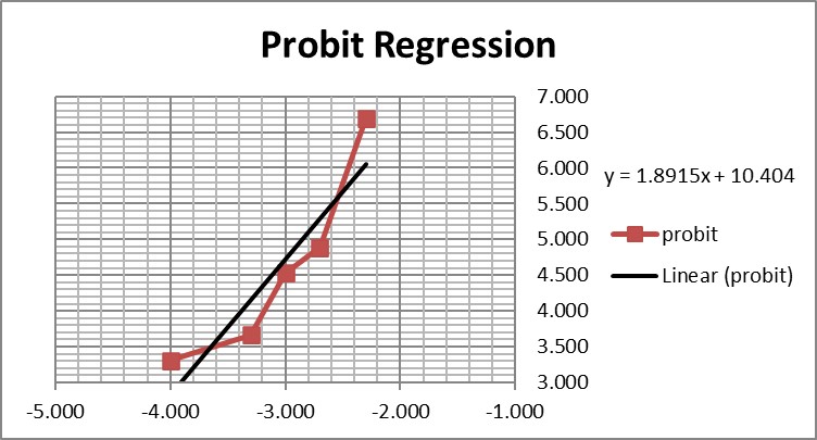
From the regression line, the calculated log C95 value is -1.990, which corresponds to a concentration of 0.010 PFU/mL. If the lowest point is removed, then the probit regression provides a better fit to the remaining 4 data points, with a line that has a slope of 2.903 and intercept of 13.1. This provides an estimate of -2.240 for log C95 and 0.006 PFU/mL for the LoD. These differences may be small, but they reveal the variability of results even for a good study that provides several data points in the probit range. Most likely the probit regression was limited to only 4 data points to provide the estimate of 0.005 PFU/mL.

Another CLSI Example

CLSI also provides a “worked example” in Appendix C [2, pages 51-53]. This example shows an initial study that included 6 different concentrations, but resulted in only 2 non-zero or non-one hit rates. Based on a review of those results, two additional levels for analyzed to provide a total of 4 concentrations with useful hit rates, as shown in the table below.

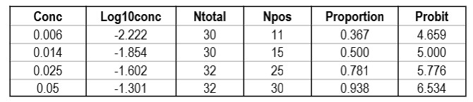
The importance of checking the experimental results to ensure a sufficient number of concentrations is an important lesson in the correct application of probit analysis.

Graphing those points is also important for demonstrating their validity for estimating C95.

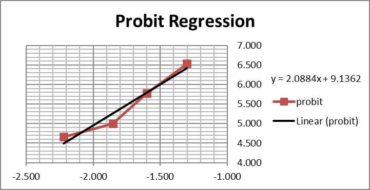
The graph is looks a little strange because of the negative log numbers, nonetheless, we can calculate the slope (2.088) and intercept (9.136), then calculate the log C95 value (-1.195) that corresponds to a probit of 6.64, and finally convert that log back to a concentration value of 0.064 CFU/mL.

For comparison, here are the results from the CLSI worked example where “the data were reanalyzed using software for probit analysis.” Here we have an entirely different regression model that fits the data to an S-shaped sigmoid curve, rather than transforming to probits and then providing a linear fit. The CLSI answer to this worked example is a LoD of 0.077 CFU/mL. Considering the differences in methodology, the answer from classical probit regression of 0.064 CFU/mL is actually in pretty good agreement with the software answer. However, as a worked example, it is not very helpful unless you happen to know what software was used and also happen to have access to that software. Rather, this example illustrates why the quality of probit analysis may be so variable, given that even the consensus guideline for good laboratory practices does not provide a standardized, detailed, workable procedure that includes the data analysis itself.

This type of probit analysis has been described in more detail by Vaks [5], who was a member of the EP17 document committee. The supposed advantages of this new mathematical model are better fit of data, better estimates with tighter confidence intervals, and fewer concentrations needed to be measured with fewer replicates. According to Vaks, because this model fits points with low detection rates of zero and high detection rates of 1.0, fewer than 3 points in the range between may be needed. The new model was compared with results from SAS PROC PROBIT, one of the most powerful statistical packages commercially available. Software for the new method was developed and copyrighted by Maplesoft, Inc., Waterloo, Canada. [Do a Google search for Vaks probit analysis to find this paper.]

What’s the point?

Probit analysis is the recommended methodology for determining the LoD of molecular methods. Unfortunately, there is no consistent practice for applying probit regression, not even in the CLSI EP17-A2 document. That means the estimates of LoD may not be reliable, even in head to head comparisons that are needed to establish the relative sensitivity of methods on the market.

Improvements are possible! First, laboratories should emphasize the collection of better data, ensuring at least 4 test concentrations provide useful probits. Second, rather than resorting to more complicated and likely proprietary statistical programs for data analysis, laboratories can implement the classical Finney methodology using an Excel spreadsheet and applying the function 5+NORMSINV(P) to convert hit rates to Finney’s probit values. Someone in your laboratory has the skills to do this and can provide reliable data analysis if you collect reliable data. Reliable data is the key to improving your estimate of LoD.

Finally, if the Excel approach is not practical, you can download log-normal probability graph paper [6] and perform these examples by hand, graphing the original data of hit rates vs concentrations directly. Let the graph paper do all the work of transforming to probits and converting to logs. You just plot the points and use a ruler to draw the best straight line through the data. The download includes 4 printable sheets for 1, 2, 3, and 4 log cycles on the x-axis. Start with the first EP17 example with the 10 data points and use the 1-cycle graph paper. For the next 2 examples, use the 2-cycle graph paper and scale the x-axis appropriately. This approach is a bit old school, but you may be surprised how well it works. And you can’t beat the cost.

References

1. CLSI EP12-A2. User Protocol of Evaluation of Qualitative Test Performance. Clinical and Laboratory Standards Institute, 940 West Valley Road, Suite 1400, Wayne, PA, 2008.
2. CLSI EP17-A2. Evaluation of Detection Capability for Clinical Laboratory Measurement Procedures. Clinical and Laboratory Standards Institute, 940 West Valley Road, Suite 1400, Wayne, PA, 2012.
3. Finney DJ. Probit Analysis: A Statistical Treatment of the Sigmoid Response Curve. Cambridge University Press, Cambridge and London, 1947.
4. 4. Loeffelholz MJ, Alland D, Butler-Wu SM, et al. Multicenter evaluation of the Cepheid Xpert Xpress SARS-CoV-2 test. https://doi:10.1128/JCM.00926-20.
5. Vaks JE. New method of evaluation of limit of detection in molecular diagnostics. Joint Statistical Meeting, Vancouver, Canada, July 28 – Aug 2, 2018. [Google search for Vaks probit analysis should give Maplesoft.com source]
6. Lognormal probability plotting paper, 1, 2, 3 and 4 cycles. https://weibull.com/GPaper/