QC Design
Patient Data or Traditional QC? Evaluating the options for QC and QC goals
Making use of data presented at the 2005 AACC conference, we demonstrate a QC application comparing the virtue of traditional QC and Patient Data QC designs. Is it best to base your QC design on data from one level of control, a 2nd level of control, or switch over to patient data?
- Recap: What do you need for QC Design?
- What data is available?
- The first QC Design with data from Control 1
- A 2nd QC Design with data from Control 2?
- What about Patient Data QC? A third QC Design
- What's the Sigma of this process?
- Reconciling the designs and/or implementing Multistage QC
- Postscript: How does this laboratory compare to others?
January 2006
Note: This QC application makes use of the EZ Rules 3 QC Design software. This article assumes that you are familiar with the concepts of OPSpecs charts, QC Design, and Average of Normals. If you aren’t, follow the links provided.
This month we highlight another poster from the 2005 AACC/ASCLS/IFCC conference, "Assessment of Total Clinical Laboratory Performance: Normalized OPSpecs Charts, Sigma-Values and Patient Test Results", (Diler Aslan, Selahattin Sert, Hulya Aybek, Gamze Can Yilmazturk, Pamukkale University, School of Medicine, Biochemistry Department, Denizli Turkey).
This paper has also been published as Aslan D, Sert S, Aybek H, Yýlmatürk G. Klinik Laboratuvarlarda Toplam Laboratuvar Performansýnýn Deðerlendirilmesi: Normalize OPSpec Grafikleri, Altý Sigma ve Hasta Test Sonuçlarý [Assessment of Total Clinical Laboratory Process Performance: Normalized OPSpecs Charts, Six Sigma and Patient Test Results] Türk Biyokimya Dergisi [Turk J Biochem] 2005; 30 (4); 296-305 (http://www.TurkJBiochem.com).
The collected data provides a good opportunity to compare the use of traditional versus Patient Data QC, as well as the virtue of using one control level or another to design your QC.
Recap: What do you need for QC Design?
For most QC design applications, you need data on routine performance of imprecision and inaccuracy. For QC design of Patient Data algorithms (also called Average of Normals, or Average of Patients), you need the ratio of the CV of the patient population to the CV of the method.
To find the quality requirements, you can make use of these online sources: CLIA, clinical, biologic.
Finally, some sort of QC Design tool will be needed, (Normalized OPSpecs charts, home-grown Excel spreadsheets, or QC Design software).
What data is available?
Diler et al. collected all the data we need on the performance of their laboratory. On a Beckman Synchron LX 20, they collected data on 22 analytes. We're going to restrict ourselves to our favorite analyte, cholesterol:
|
Control 1
|
Control 2
|
|
| Level | 102 | 221 |
| Bias % | 1.0 | 0.5 |
| CV | 1.6 | 1.4 |
They also calculated the CV of the patient variation, with an N of 671 patients, at 20.7. The resulting ratio of CV of the patient population to the method variation of the controls is 12.9 and 14.8, respectively.
As for the quality requirement: CLIA sets a goal of 10% for proficiency testing performance.
The first QC Design with data from Control #1
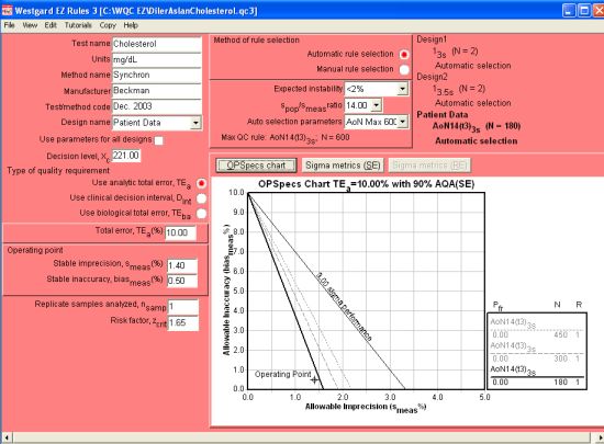
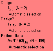
We make use of EZ Rules 3 here not only because of its automatic QC selection, but its expanded capability to design QC for multiple levels and mutiple quality requirements. In the form mode, all of the different goals and performance data can be entered and observed:
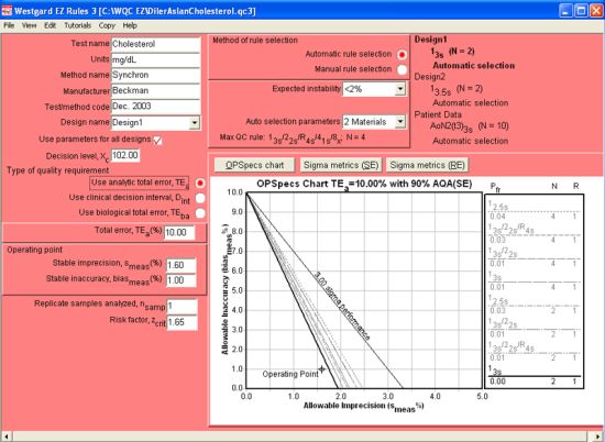
The figure above displays the graphs and automatic QC selection for the Level 1 control (at 102 mg/dL) using an analytical quality requirement. The Design name drop-box (located in the upper left part of the screen) controls the display of the current QC Design. So, when it is set to Design1, it is showing the data and control rules for Level 1. Note that performance is so good that the rule selected is a 13s control rule with 2 control measurements.
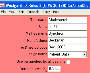 When using the EZ Rules 3 form mode, descriptive data is first entered in the top left corner of the window (Test name, Units, Method name, etc.). Then, further down, you select the type of quality requirement (in this case, (Use analytic total error, TEa). Once that is selected, further below on the left side, you can enter the Total error, followed by the Stable imprecision and Stable inaccuracy.
Next you go the top of the middle of the screen, and select how you want to choose the rules (Automatic selection is easiest), choose the level of expected instability (choosing <2% indicates the instrument is very stable), followed by the Auto selection parameters, where you specify the number of control materials (for 2 controls, you select 2 materials, 3 controls, 3 materials, etc.) For this instrument, 2 controls are being used.
Once you select 2 materials, the Automatic selection engine is engaged, and the OPSpecs chart will display the recommend control rule and number of control measurements:
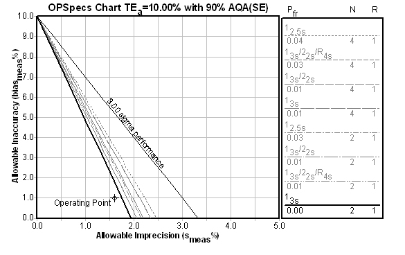
2 controls with 3s limits is definitely good news. But this is based on the data from one control - what does the data from the other control say?
A 2nd QC Design for a 2nd Level of control?
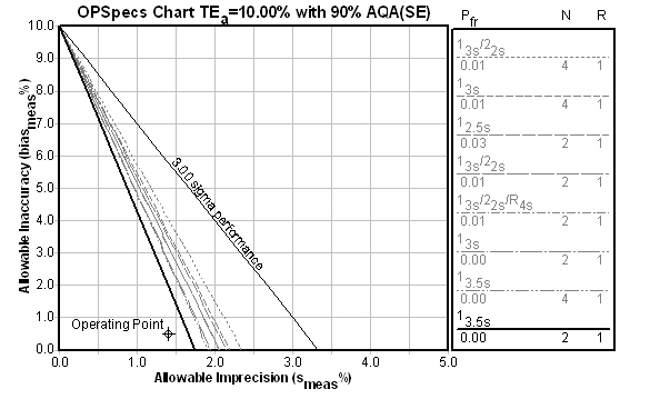
If we set up a 2nd QC Design (selecting Design2 from the Design name dropbox), we can enter the performance of the Level 2 control (at 221 mg/dL). The resulting evaluation is still excellent:
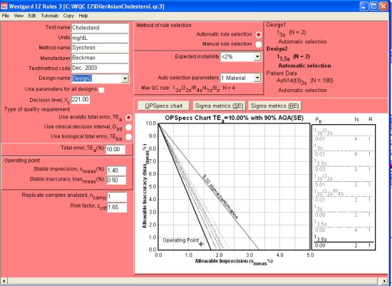
In fact, if we use the Level 2 as our critical decision level, we could consider using a 13.5s control rule with N=2. In previous QC applications for cholesterol, we have preferred critical decision levels around the 200 mg/dL level, since that is usually where differences in the test value can produce significant differences in diagnosis and treatment.
What's the Sigma of this process?
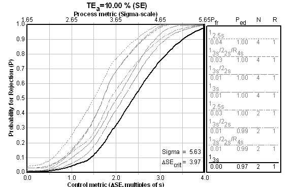
Is there a reason both controls are giving wide limits and minimal Ns? Yes. That reason is made obvious when the Sigma metrics / Critical-Error charts are consulted (the chart below is the Level 2 control, followed by a chart for the Level 1 control) :
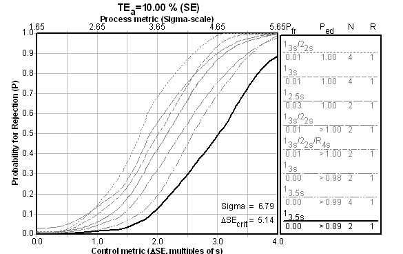
The fact is, if you achieve higher than Six Sigma, it doesn't matter which QC Design model you use - you just need to do the minimum amount of QC. Even if we look at the performance of the first control level, performance against the universal benchmark is good:
What about Patient Data QC? A Third QC Design
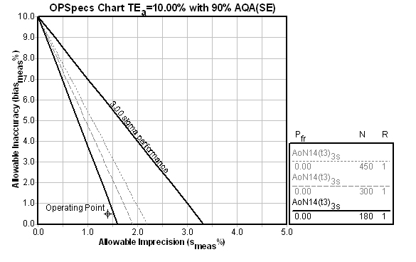
 When we move on to the third QC design - Patient Data - we need to consider the spop/smeas ratio, which we have already stated was calculated at between 12.9 and 14.8. The software program gives us the choice of 13.0, 14.0, 15.0, etc., so that is the selection we will make. We must further select the maximum number of patient samples we are willing to run to calculate the Average of Normals (you have a choice of up to 450 patients depending on the ratios and performance). In this case, we select 600 patients as the maximum we'll run. Luckily, we won't have to worry about collecting that many samples:
Here you can see that Average of Normals rules have a different nomenclature that the usual statistical limits. [Briefly: AoN means Average of Normals; the 14 indicates the ratio of spop/smeas; t3 means truncation limits are set at 3s to exclude data from the Average of Normals calculation; and 3s means the control limits are set at 3s after the calculation] The selected control rule has an N=180, which means that 180 patient samples are required for the calculation.
Reconciling the designs (and/or implementing Multistage QC)
In the end, the performance of this instrument is near Six Sigma, and no matter what data or what QC Design model you would use, the answer for traditional QC is basically the same: few controls, wide limits. For all that complexity in design, it's a very simple recommendation. Given that fact, you may not want to even consider Patient Data QC as your method of controlling the test. There is very little to worry about or argue over for this method. So breathe a sigh of relief. Congratulate yourself on selecting the instrument and operating it correctly. And move on to the next problem.
 One possible use of these multiple QC designs remains: if you are a more sophisticated lab and still want to use Patient Data QC as the main way to monitor this method (and reduce your use of controls), the different designs will help you set up a Multistage QC design. That is, you will make use of traditional QC (with controls) during start up or critical stages of less than stable performance, until the point at which you have gained enough patient samples (here, 180 samples) to calculate the Average of Normals. Then, when your Average of Normals begins to indicate a problem, you can put controls on the instrument, using the QC Design previously recommended, to confirm that there is (or isn't) a problem.
Postscript: How does this laboratory compare?
Up until this point, a reader may accept this data as a sign of superior laboratory performance, but reserve the right to believe this is an exception, not the rule. Now that we've established what this laboratory has accomplished, let's place it in the greater context of other laboratories.
On the OPSpecs chart below, we plot not only the performance data supplied with the Beckman Synchron specifications (Instructions for Use, available on their website), but also the most recent data from the (2005 January) New York Wadsworth proficiency testing event of 37 Synchron LX 20 instruments, as well as the NCEP recommendations for precision and accuracy of cholesterol methods.
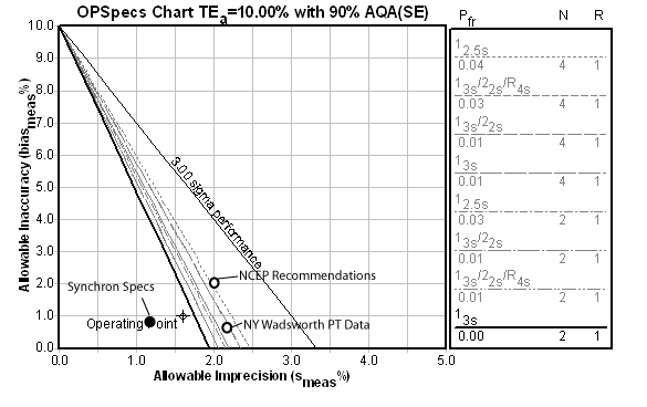
As you can see, the laboratory is performing slightly worse than the instrument specifications (not surprising, since manufacturer specifications are often calculated with data produced in ideal situations). Yet they are still peforming better than the NCEP recommendations and the NY PT participants. So they are "above average."