Z-Stats / Basic Statistics
Z-2: An Organizer Of Statistical Terms (Part I)
Madelon F. Zady
Dr. Zady introduces all the terms of statistics. If you don't know your t-tests from your F-tests, this is a painless place to start.
EdD Assistant Professor
Clinical Laboratory Science Program University of Louisville
Louisville, Kentucky
April 1999
- Average - the most common statistic
- Standard deviation - a common laboratory statistic
- Probabilities or p's - where statistical discomfort begins
- z-score - a combined statistic
- t-test - significance of a difference between means
- F-test - a test of significance that drops the square root
- Review of the organizer
- Author biography
[Lessons 2 and 3 provide a somewhat over-simplified description of the rest of this series. This is done to aid the learner in learning statistical terms and concepts. The lessons are designed to serve as an "organizer" for the coming material. If you are familiar with these statistical terms and concepts, you can quickly review this lesson (and lesson 3) and get ready for more detailed materials in Lesson 4 (coming soon).]
 In prior statistics classes, you may have learned about important terms such as xi's, x-bar's, SD's, p's, z's, t's, F's, r's,a's, b's, and sres's. How much do you remember about these concepts? Perhaps you have never had a formal course in parametric statistics, but have run across these terms on computer printouts in your laboratory QC work.
It is important to understand the statistical concepts if you are to have power over them. In that way, you can use them to make needed modifications to your QC systems and to understand future changes in the approach to QC systems.
Lessons 2 and 3 provide a "statistics organizer" for common statistical terms and concepts. In subsequent lessons we will explore each concept in detail and also its relationships to QC. You will be able to understand the concepts without performing math exercises. As you gain the perspective, you may want to challenge yourself with some problems and can use available computer programs to perform the calculations. Or use the tools available on this website.
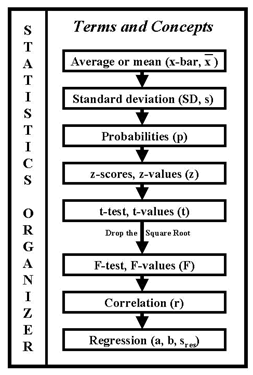
The discussion in the next two lessons is centered on the accompanying figure, which I call an "organizer" because it arranges the statistical terms and concepts in an order for learning. One of the secrets to learning statistics is to realize that all of these statistics are related and that the terms build on one another, as shown by the vertical arrows. Each new layer builds upon the principles of the prior layer.
Average - the most common statistic
The simplest term is the average or mean, which is commonly used by almost everyone in our society. Given a series of numbers that show some fluctuation, or variation, the best description of what has been observed is the average of those numbers. An example in the laboratory is the calculation of the average for a group of measurements on a control material. The average is the best estimate of the value that is to be expected on continued measurements. It is also your best bet, if you were asked to guess a number!
Standard deviation - a common laboratory statistic
The next term is the standard deviation, or SD, which is familiar to most laboratorians. In statistical QC, control limits are calculated from the mean and the SD, usually as the mean +/- 2SD or the mean +/- 3SD. When control limits are set as the mean +/- 2SD, it is expected that 19 out of 20 control measurements will fall within the limits because the limits encompass 95% of the area under a bell-shaped or normal curve, as shown in the second figure. When control limits are set as the mean +/- 3SD, it is expected that 99 out of a 100 control measurements should fall within the control limits, because they encompass 99.7% of the area under the normal curve.
The SD is determined by analyzing many aliquots of a control material (at least 20), calculating the mean by adding the values of all of these and dividing by N (here 20). Then the mean value is subtracted from each of these values (control value - mean) and this latter value is squared and summed (?) across all 20 [? (control value - mean)2]. This value is divided by 20-1 or 19. Then the square root is taken. This "value - mean" (value minus the mean) term will be a recurring theme in statistics. The calculation of SD will be more fully explained in the coming lessons. (See also QC-The Calculations.)
Probabilities or p's - where statistical discomfort often begins
The third term is probabilities. When we discussed the use of the SD in quality control, we stated that we usually want the values of our control runs within +/- 2SD of the mean of the control material. That +/- 2SD comprises 95% of the area under the normal curve around the mean of the control material. Simply said, if the control value falls in the 95% area, then it has a 0.95 probability of not being statistically different from the mean. Said another way, there is a 0.95 probability that the control value is "the same" as the mean. If the control value falls outside this 95% area, into the 5% of the area that makes up the two tails of the curve, then the control value has less than a 0.05 probability of being statistically the same as the mean. Said another way, there is only a 0.05 probability that the control value is "the same" as the mean. Probabilities as they relate to the normal curve distribution will be covered in a future lesson.
z-score - a combined statistic
To understand the z-score, we need to look more closely at the familiar SD. In its original definition, SD was described in concentration units, i.e., the SD may be 5 mg/dL for a cholesterol control whose mean value is 200 mg/dL. Control limits for 2 SDs would be 190 to 210 mg/dL, or +/- 10 mg/dL. When we describe control limits in the context of +/- 2SD, we are really using the standard deviation as a standard score. Standard scores express the difference between a value and the mean of the control material as a multiple of the standard deviation, i.e., how many standard deviations are in that difference. The most universal of all the standard scores is the z-score, which is used on some recent QC analytical systems. This z-score may cause confusion, especially for analysts who have been around the laboratory for a long time. It is important to realize that the +/- 2SD rubric that you have been using for years and years is actually a z-like or standard score.
One of the very practical uses of a z-score is to compare different distributions, so you do not have to be concerned about any particular mean or SD value. Suppose you were analyzing two different control materials and wanted to compare results on consecutive measurements. Now instead of comparing each control value with the mean of that control, you can take the difference of each control from its own mean and then divide by its standard deviation to tell how far each value is from its respective mean. A z-value of 2.4 would indicate the control value is 2.4 "SDs" above its mean. Notice here that the z produced is a decimal fraction. With z-scores, we are no longer limited to just ±1, 2, or 3. And also notice that a z of 2.4 would indicate that this control value lies in the tail of the distribution or outside the 95% area of the curve. If the z-value on the next observation on the other control material were 2.1, you have evidence that both controls are running high, greater than 2 "SDs" above their respective means. Remember, because the z-score is calculated by dividing the difference between the control material and its mean by the SD, +/- 2z's will give 95% of the area under the bell-shaped or normal distribution.
You can also use z-scores to compare the monthly mean observed on a given control material to the means observed for earlier months. In this comparison, you would be using an SD calculated from the monthly mean values (which is often called the standard error of the means). Just as before, if the mean of the current month falls within ±2SDs of the mean of the distribution of monthly means, then it falls within the 95% area under the curve and there is a 0.95 probability that the current month's mean is "the same" as those observed for earlier months. If the current mean is greater than 2SDs from the prior mean (or in the tails of the distribution) then there is only a 0.05 probability that the current mean is the same as the prior mean. Note that while laboratorians often use the term SD here as a standard score or z-like term, it is actually the standard error of the mean that is most often used to produce a z-score. These error terms will be covered in a future lesson as will sampling distributions of means.
t-test - the significance of a difference between means
An understanding of t-values comes from looking at the prior terms. z-scores have their own bell-shaped distribution based upon the mean (µ or mu) and standard deviation (s or sigma) of a large population. (Greek symbols are used to describe parameters for large populations, whereas regular alphabetic conventions are used for the statistics calculated from samples of these populations.) For z-scores to be determined and used, the mu and sigma of the entire population must be known, which often is impossible for real applications. Fortunately there is another family of z-like scores called t-values that have a nearly normal distribution when sample sizes are relatively small. The population mean and sigma do not have to be known to use these t-distributions, and the interpretations are the same.
For example, the difference between the mean of the current month minus the mean of the prior month can be divided by an error term, like an SD, to calculate the multiple of SDs between the means. The number obtained now is called a t-value. If the current mean is within +/- 2ts of the mean of the prior month then it lies in the 95% area or there is a 0.95 probability that it is "the same" as the prior mean. If the current mean lies in the 5% area of the tails then there is a 0.05 probability or less that the means are "the same."
As an example application, t-values are used in experimental designs when a researcher is attempting to show that a group of treated animals will have longer mean life spans than a group of untreated control group animals. The mean life spans of these two groups will be compared through a t-statistic. t-values are also used in method validation, particularly in the comparison of methods experiment to assess whether the means obtained for an analyte are the same on instrument A and instrument B. More will be said in a later lesson.
F-test - a test of significance that drops the square root
Beginning with the second statistic in the organizer - the SD, we have been dealing with terms that involve a square root. All of these error terms are calculated by taking the observed values and subtracting the mean value, squaring the difference terms, adding the square terms, dividing by N, and finally extracting the square root. The SD, z-score, and t-test all involve a term with a square root. The next concept, F, does not use the square root of its error term, and that important fact is noted in the organizer. Sometimes a statistical design can use either a t or an F statistic. The results and conclusions will not be the same unless you realize the F = t2 or t=(F)1/2.
The point is that t's and F's are related. However, F is an improvement on t when you are trying to test more than one mean against another's distribution. For example, F is preferred over t if a researcher were trying to test the effectiveness of four different levels of an antibiotic to see which would be most effective, or if a laboratorian were testing the means obtained on an analyte using three different screening instruments. In the first example, at least four t-tests could be performed, in the latter example at least three t-tests. However results from these statistical tests could become a problem. We call this problem Type I error, and it will be covered later. The F-test, more commonly referred to as ANOVA (or other OVA testing) can control the introduction of statistical error in these experimental designs or method comparisons. Usually these tests are computerized, but the interpretation follows the same general pattern that we have seen above. F has its own distribution. If the F result is within "+/- 4Fs" then the values lies within the 95% area of the F-distribution, and there is a 0.95 probability that the means are all "the same." If the F result is greater than "+/- 4Fs" then the value(s) lie in the tails of the F-distribution, and there is only a 0.05 probability or less that the means are "the same." More will be said in a later lesson.
Review of the organizer
As we move through the statistical concepts discussed above, we see that each successive level builds upon the previous one. Means or averages are the starting point and describe the most likely location of a value. Standard deviations provide additional information about the distribution of values about the mean. Knowing the mean and SD allows some inferences about the probabilities of certain events occurring. These probabilities can also be related to "standard scores," which describe the relative location of values within the normal distribution. You can think of the standard score as a "gate" on the normal distribution. The gates placed at +/- 2 standard scores enclose 95% of the area under the curve. If a new value falls within this area, then it has a 0.95 probability of being "the same" as the mean of the distribution. If the value falls in the 5% area that comprises the tails, it has a 0.05 probability or less of being "the same" as the mean of the distribution. z-scores are the common statistical form for standard scores. t-values provide a more practical form for testing the difference between two mean values. F-values are related to t-values (remember by dropping the square root) and permit testing the differences between multiple means or averages.
Don't let these statistics overwhelm you. The "organizer" will help to keep them straight and will help you to learn the nomenclature and understand how the terms build on each other. The next lesson will consider statistical relationships and expand the organizer to include correlation and regression.
Biography: Madelon F. Zady
Madelon F. Zady is an Assistant Professor at the University of Louisville, School of Allied Health Sciences Clinical Laboratory Science program and has over 30 years experience in teaching. She holds BS, MAT and EdD degrees from the University of Louisville, has taken other advanced course work from the School of Medicine and School of Education, and also advanced courses in statistics. She is a registered MT(ASCP) and a credentialed CLS(NCA) and has worked part-time as a bench technologist for 14 years. She is a member of the: American Society for Clinical Laboratory Science, Kentucky State Society for Clinical Laboratory Science, American Educational Research Association, and the National Science Teachers Association. Her teaching areas are clinical chemistry and statistics. Her research areas are metacognition and learning theory.