Z-Stats / Basic Statistics
Z-7: Hypothesis Testing, Tests of Significance, and Confidence Intervals
Hypothesis testing, tests of significance, and confidence intervals - here are three more statistical terms that strike fear in the hearts of many laboratory scientists! If you survived the previous lesson on probability, then you can also get through this lesson. The ideas presented here will be very helpful in making good decisions on the basis of the data collected in an experimental study.
EdD, Assistant Professor
Clinical Laboratory Science Program, University of Louisville
Louisville, Kentucky
September 1999
- Hypothesis testing - what's "the same" and what's "different"?
- Tests of Significance and the Student t-test
- Confidence intervals
- A note about the "paired t-test" for comparison of methods
- About the Author
Hypothesis testing, tests of significance, and confidence intervals - here are three more statistical terms that strike fear in the hearts of many laboratory scientists! If you survived the previous lesson on probability, then you can also get through this lesson. The ideas presented here will be very helpful in making good decisions on the basis of the data collected in an experimental study. Remember that the reason we collect data is to make some decision, e.g., the precision of a new method is acceptable, there is no systematic difference (bias or inaccuracy) between a new method and a comparative method, the reference intervals for males and females are the same, etc.
Hypothesis testing - what's "the same" and what's "different"?
There are two groups of mice each with 50 members. Both groups are actively infected with the same organism. Group A - the experimental group - is treated with an antibiotic. Group B - the control group - is not treated. Intuitively, we expect the life span of the group receiving the antibiotic (A) to differ from that of the control group (B). To experimentally prove whether or not the antibiotic is effective, we measure the life span in days, average the results for each group to give a mean life span, compare the mean life span of group A with that of group B, and determine whether the mean life spans are the same or different. This determination is carried out by hypothesis testing and a statistical test of significance - the main topics of this lesson.
Hypothesis testing makes use of the unit normal distribution that was discussed in the previous lesson, which emphasized the use of z-scores to draw some conclusions. Z-scores are calculated from the true population parameters mu and sigma. In many experimental situations, we don't actually know the true population mu and sigma, therefore we can't use z-scores. However, we can usually calculate the mean and standard deviation of our groups, calculate t-scores or t-values, and use the t-distribution or Student's t-test to test hypotheses. The discussion here focuses on the t-distribution and the t-test, but the principles and procedure also apply to other statistical tests of significance.
Answered by a Straw Man called Ho
In analyzing the data, we actually begin by assuming that the mean life span of group A (experimental group) is the same as that of group B (control group). Or, life span of A = B or A-B = 0. In this way, the experimenter sets up a "straw man" hopefully to be knocked down by the resultant data. This is called a null hypothesis (Ho) and is symbolically represented as shown below:
![]()
There is also an alternate hypothesis (Ha) that assumes the means of the two groups are not the same, in which case they must be different:
![]()
In all likelihood, the researcher wants to establish the fact that the antibiotic works (especially if the research is funded by a pharmaceutical company). The goal here is to unseat the "straw man" by rejecting the null hypothesis, in which case the alternate hypothesis must be true, i.e., there is a difference. However, academic and clinical integrity demand that the conclusion be based upon rigorous analyses of the data. In this case, what would make the experimenter comfortable enough to reject the null hypothesis? How different would the mean life-spans of the two groups have to be to conclude they are not the same?
"The same" means Ho is left standing
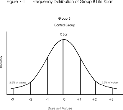
 Figure 7-1 shows the frequency distribution of life spans for Group B (the control group). The frequency is shown on the y-axis and the life span in days is shown on the x-axis in terms of a standard score, such as ±1, ±2, and ±3. Remember from the previous lesson that a standard score such as z-value requires knowledge of the true population mean and standard deviation, whereas a t-score can be calculated from the observed mean and SD for a group of any size. In this application, only a t-score can be calculated to describe the location of individual life spans relative to the average or mean life-span of the group. The same is true for Group A - only t-scores can be calculated from the available data.
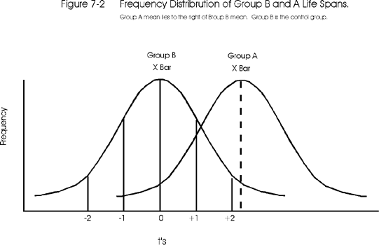
Figure 7-2 below shows the frequency distribution for Group A (the experimental group) superimposed onto that of the control group, in this case using the t-scores that are calculated from the observed mean and SD of the experimental group. From the Figure 7-2, it can be seen that Xbar A (the mean of the experimental group) is contained in the area which is greater than 2 t's above the Xbar B (the mean of the control group).

"Different" means Ho has been knocked down
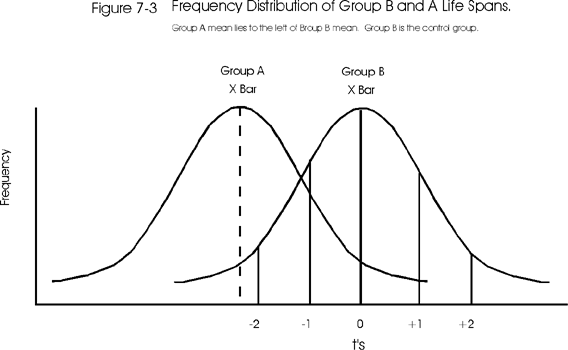
Figure 7-3 shows the opposite situation in which group A's mean is greater than 2t's below Xbar B. Considering the unit normal curve, ± 2z (here ± 2t) encloses 95% of the distribution. Since the mean of group A is out of this 95% area, there is a less than a 5% chance that these two means are the "same," or a less than 0.05 probability that the mean of group A occurred "by chance" and could really be part of the control group's distribution. Is the researcher comfortable enough with this probability to reject the null hypothesis of no difference between the means? Would it be better if the difference were at ± 3t which would give a less than 0.001 probability (or 0.1% chance) that the two means were the same? The answer depends upon the experimental design and the research tradition. In medicine, very often probabilities for rejecting the null hypothesis are in the range of 0.001 or even less.

Tests of Significance and the Student t-test
A test of significance is a statistical test that attempts to determine whether or not an observed difference indicates that a given characteristics of two groups are the same or different. The equation for a test of significance has the general form: test statistic equals the observed difference divided by expected experimental variation. In the context of the discussion above, a t-statistic can be calculated from the observed difference between two means divided by a measure of the expected experimental variation, such as the standard error of a mean. This lesson will focus on the Student t-test, but there are other tests of significance that are similar in form and procedure. The Student t-test is perhaps the most common and most useful test of significance, therefore it serves as the best illustration. (By the way, Student is actually the pen name for the mathematician who develop this test and whose real name was Gosset. Why would anyone want to be called "student" for the rest of his life?)
General procedure
- State the hypothesis. To answer the question whether the means of group A and group B are the same or different, they are first hypothesized to be the same. The null hypothesis is stated as Ho: XbarA = XbarB or XbarA - XbarB = 0. The alternate hypothesis is stated as Ha: XbarA … XbarB.
- Set the criterion for rejection. How different must these means be in order to say that the mean of group A does not belong to the B group (control group) distribution? Suppose a researcher decides that a difference of ± 2t (or a mean difference greater than the 95% area) would be critical. Using a t-distribution the value is actually ± 1.96 t, but we often round this to ± 2t. If the mean of group A appears to be ± 2t away from the mean of group B, then there is only a 5% or less chance that the group A mean belongs to group B. This 5% describes the area of the unit normal curve or the t-distribution with large N that is outside the criterion for rejection, in this case 0.05 of the area is outside ± 2t's. This area of rejection for the null hypothesis (demonstrating that the means of both groups are not the same) is the 2.5% on the right side of the curve and in the 2.5% on the left side of the curve. (See Figure 7-1.) The 0.05 level is also called the alpha level or level of significance, which can be set to be more or less stringent, e.g., 0.001, 0.01 or even 0.10.
- Compute the test statistic. The idea is to see just how many t-units group A's mean is away from group B's mean. To do this, we calculate a t-value that is called tcalc or t-calculated, as follows:

Note that this equation has the same "form" as we saw before with the z-score formula. The difference between the two means is expressed in terms of the number of standard deviation units, in this case the units are the standard error of the mean. - Decide about Ho. In our earlier example where the superimposed frequency distributions of the two groups were examined, a judgement call about the two means was attempted by merely considering the ± 2t distance. This was a crude estimation because the shape of the distribution was not taken into consideration. And usually we do not have the luxury of superimposing graphs and being assured of completely normal distributions. Instead, we compare our calculated t-value to a critical t-value, which we look up in a statistical table. If the calculated t is less than the critical t, the null hypothesis is accepted and we conclude that the means are "the same." If the calculated-t is greater than the critical-t, the null hypothesis is rejected, in which case the alternative hypothesis must be true and we conclude that the means are "different."
Table of critical t-values
Although we routinely use computer programs to perform t-test for us and provide both the calculated and critical t-values, it should be helpful to see how a t-table is used manually. As indicated in Lesson 6, the t-distribution is actually a family of distributions whose shape changes dependent upon the degrees of freedom (df) which are related to the number of subjects in the group (N'). The larger the N, the more normal the distribution. A t-table provides the critical t-values (tcrit) for the number of df's in the groups and the level of significance or alpha desired (which is selected in step 2 and is to set the criteria for rejection). Click here to see a table of critical t-values.
To find the tcrit, from the table, locate the desired alpha level in the column heading and the df's in the row, then use these as coordinates on the table and read across and down to find the tcrit. At alpha = 0.05 and a large N (bottom rows), the tcrit approaches ± 1.96 or approximately 2.0. So, when N is large, the situation appears very much like the z-score/unit normal distribution that we saw before. If alpha=0.05 and df=40, tcrit is 2.02; for df=30, tcrit is 2.04, and for df=20, tcrit is 2.09. Therefore, our approximation of 2.0 begins to breakdown as df becomes 30 or less.
If tcalc happens to compute as say 1.45, then it does not exceed tcrit and lies inside the 0.95 area. Strawman Ho is left standing, signifying there is no difference. The probability is that A group's mean belongs to the B group distribution or they are statistically the "same."
If tcalc happens to compute as say 3.56, and tcrit from the table is 2.00 or less, such results indicate that tcalc is located in one of the tails of the distribution or in the 0.05 area. Strawman Ho has been knocked down and we conclude there is a difference between the two means. The probability is 0.05 or less (p=0.05 or less) that the mean of the experimental group A is found is the same distribution as for the control group.
Confidence Intervals
Oftentimes the confidence interval (CI) is listed as the 5th step in hypothesis testing. Once a t-test is performed, the range of mean values can be established so that any future group mean can be compared to these and declared "the same" or "different." For example, given the example experiment for testing an antibiotic, what range of life-span means for future tests of group A would be considered close enough to group B's mean life span such that Ho would not be rejected? This question can be answered by calculating the confidence interval around the mean life span of the control group (B), as follows:
CI = Xbar B ± (tcrit)(sXbar)
The value for t is looked up in the t-table and the upper and lower limits are calculated by adding or subtracting a multiple of the standard error of the mean. The confidence interval is simply back-tracing the steps of the t or z-score determination to "re-inflate" the score to it's original "concentration" units. (But here we are using days instead of mg/dl.) Since these days will be added to or subtracted from the mean days for the control group, this mathematical expression gives the range of days in which the researcher can be 95% confident that the mean of the control group lies. And, this formula will give the range of mean days that group A could live and still belong to group B (control group). In other words, the formula indicates that, if group A mouse population dies somewhere inside this CI range of days, the antibiotic did no good.
This quick treatment of a confidence interval is somewhat oversimplified and will be expanded on in latter discussions. The point here is that tests of significance and confidence intervals are related and provide complementary information. Laboratorians often find confidence intervals to be more meaningful than tests of significance because the uncertainty of an experiment can be expressed in concentration units (which are understandable) rather than statistical units.
A note about the "paired t-test" in method comparison
The example discussed in this lesson pertains to an experiment where there are different individuals in the sample and control groups. In method comparison studies where the same samples from individuals can be analyzed by two different analytical methods, the t-test can be applied to the pairs of results from the different samples. The same general steps apply for this paired t-test, but note the following:
- The inaccuracy or bias between the methods is estimated as the difference between the average of method A and the average of method B, which will be the same as the average of the individual differences.
- The experimental variation is estimated by the standard deviation of the differences, which is calculated as follows:
SDdiff = [S(yi - xi - bias)2/(N-1)]1/2 - The t-value is calculated from the bias, SD of the differences, and the number of paired samples (N) as follows:
tcalc = (bias/SDdiff)N1/2
*** Remember that raising a term to the one-half power is the same as taking its square root.
Just a note: There is a very different outcome desired for Ho depending upon whether he is in an experimental design or a method comparison. In experimental design, we want to show that there is a difference between level means (so we want to knock Ho down). In method comparison, we usually want both the means to be the same (so we want Ho to remain standing)
About the author: Madelon F. Zady
Madelon F. Zady is an Assistant Professor at the University of Louisville, School of Allied Health Sciences Clinical Laboratory Science program and has over 30 years experience in teaching. She holds BS, MAT and EdD degrees from the University of Louisville, has taken other advanced course work from the School of Medicine and School of Education, and also advanced courses in statistics. She is a registered MT(ASCP) and a credentialed CLS(NCA) and has worked part-time as a bench technologist for 14 years. She is a member of the: American Society for Clinical Laboratory Science, Kentucky State Society for Clinical Laboratory Science, American Educational Research Association, and the National Science Teachers Association. Her teaching areas are clinical chemistry and statistics. Her research areas are metacognition and learning theory.