Z-Stats / Basic Statistics
Z-11: Confidence Intervals
How much do you trust the numbers your laboratory produces? There's a statistical way to determine just how much.
EdD, Assistant Professor
Clinical Laboratory Science Program, University of Louisville
Louisville, Kentucky
July 2000
- Review of us of Confidence Interval (CI) in hypothesis testing
- Use of CI in parameter estimation
- Theoretical sample distribution and the Central Limit Theorem
- Confidence Intervals around zero
- Summary and review
Our prior discussion concerning confidence intervals (CI) in Lesson 7 was somewhat over simplified. While we adequately addressed the purposes of using confidence intervals in the clinical laboratory QC program, the theoretical coverage was sparse. This section is intended to align the practical and theoretical, however some conceptualizations will remain unexamined because they are beyond the scope of these lessons.
Review use of CI in hypothesis testing
Recall from the earlier mouse-antibiotic experiment, the 95% confidence interval was expressed as:
CI = control group mean ± (tcrit)(sXbar)
where tcrit at an alpha of 0.05 is 1.96 or approximately 2.00 and sXbar is the standard error of the mean or SE covered in Lesson 5. In this case, the control group mean was used as if it were a population mean. This CI formula essentially set up a ±2 t interval on the curve surrounding the control group mean. The formula also re-inflates the t-value to a "concentration" value, here days of life span. It was further stated that we could accept the mean of any new experimental group as being the "same" as the control mean if the new mean fell into this CI or days of life span.
Use of CI in parameter estimation
As it turns out, there are a couple of ways of looking at confidence intervals. CI's have different meanings depending upon whether they are used in hypothesis testing (as above) or in parameter estimation such as estimating a population mean. Since we already looked at hypothesis testing, the following is an example of parameter estimation.
Suppose the population mean is unknown but conjectured or assumed to be some number. A simple sample of certain N is drawn from this population that has an unknown mu. The mean is calculated for this sample resulting in Xbar, as well as an error term such as the SE or sXbar. Since the mean for the population is unknown, the mean of the sample from the population is the best one-point estimator of the population mean. The CI is set up around this Xbar using the formula above for a 95% confidence interval. Remember this confidence interval is set up around the sample statistic or a single sample mean and not around the population parameter. In this case the interpretation would be that there is 95% confidence that mu or the population mean resides in this interval around the single sample mean.
The chain of reasoning is as follows:
- Assume or hypothesize a mean for a population, for example mu = 100. The null hypothesis becomes Xbar - 100 = 0.
- Draw a sample and calculate the mean or Xbar.
- Perform the t-test to see if the Ho can be overturned.
- If Ho is retained, set up the confidence interval around the sample mean using the following formula: CI = sample mean ± (tcrit)(sXbar)
- If a 95% confidence interval is desired tcrit = 1.96. The 95% CI just represents the 95% area under the normal curve distribution with 5% of the area in the two tails. Suppose the values were determined to be as low as 86 and as high as 114. There is 95% confidence that the mean of the population resides in this interval.
Theoretical sampling distributions and the Central Limit Theorem
 It is obvious that chance would play a great role in the above calculation. If another sample were taken from the above population, it is quite likely that an entirely different Xbar would have been obtained. That Xbar would have affected the upper and lower limits of the 95% confidence interval. If five different samples were pulled, they could each have different Xbars and different CI's, as shown in the accompanying figure. There is a 95% chance that the "true" or conjectured population mean resides in each of these intervals.
Of course there are many more than just five possible samples in the population. Remember in Lesson 5 when we were trying to determine the standard error of the mean, we pulled twelve samples. Then we talked about the sampling distribution of the mean that contained all possible sample means. In order to increase the chance of capturing the true mean of the population, all possible sample means and all possible confidence intervals would have to be determined. It could take a great deal of effort and time to do this.
Fortunately, it is not necessary. Statisticians use theoretical sampling distributions instead that are defined by mathematical theorems. The theorems provide information about the shape, central tendency and the variation of these distributions. The shape of the sampling distribution of the means is defined by the central limit theorem. The Central Limit Theorem tells us that, as the size of N increases, the sampling distribution of means approximates a normal curve. This happens even if the distributions from which the samples were taken are not normal! Regardless, the distribution of their means will be normal. (The theorem also applies to differences in means and other statistics.)
This is a tremendous boon to those of us who are used to putting gates on the normal distribution. If we stick with the sampling distribution of the mean, the standard error term and the central limit theorem, we can always use our ±1.96 gates. The calculation of all possible sample means and their subsequent normal curve distribution or the Central Limit Theorem means that theoretically 95% of sample means from this population lie within ±1.96 standard errors of the true population mean, and the same type of generalization would apply to their confidence intervals. Remember the sampling distribution is always normal.
In hypothesis testing, with a known population mean, the Central Limit Theorem and the theoretical distributions are also used. When Ho is rejected, the sample mean is not expected to lie in the confidence interval around the population mean. When Ho is retained, the sample mean is expected to lie in this confidence intervals.
In a laboratory comparison of method experiment, we can continue to think of setting up the 95% confidence interval around the original test procedure mean in order to determine whether the new test procedure mean is within that interval. However, we should remind ourselves that we are assuming that the mean of the original procedure is functioning as the mu for the population. We must acknowledge that we are working with a theoretical sampling distribution.
Confidence intervals around zero
If we really want to be statistically correct, we must also realize that we are dealing with the differences in means. In Lesson 8, we corrected some of our ideas about statistics by considering the two-sample case. During the first part of this lesson we have been discussing the difference between the means of one method and the mean of the population. In actuality, when we consider comparing method means, we are discussing the difference between two sample means and their difference from their own population means. That is, there are two samples X and Y. These two samples came from their respective populations X and Y. We need to think about subtracting the difference between the population means from the difference between the sample means, i.e., [(Sample mean Y - Sample mean X) - (mu Y-mu X)].
The formula for tcalc that we used in Lesson 8 was the difference in means formula:
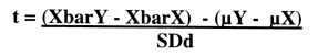
The null hypothesis is: (XbarY - XbarX) - (µY - µX) = 0.
Then we hypothesized the difference in (µY - µX) to be zero, so the formula became:
And the null hypothesis is: (XbarY - XbarX) - 0 = 0.
 The next figure shows the theoretical sampling distribution of the difference between means. Using the theorem, the sampling distribution of the difference between means is normally distributed with zero at its mean. If the tcalc for any set of differences in means resides within the 95% gates on this curve, then the means are considered "the same." Now all that remains for our method comparison is to see if the difference between the method means is zero, and the Ho would be retained. We could also take a short-cut and say that if zero lies within the confidence interval of the difference between method means then we can accept their difference to be zero. The formula for the CI should seem familiar:
CI = (XbarY-XbarX) ± (tcrit ) (SDd)
Now if samples of Y's and X's were chosen and the difference between their means was determined, the 95% confidence interval could be depicted as we see on the sampling distributions in 2nd figure. Since the 95% confidence interval contains the number zero, the null hypothesis of no difference cannot be overturned. The test procedures are considered to give similar results.
If the result appeared as in the 3rd figure below, the CI does not contain the hypothesized value of zero. It is obvious that the null hypothesis would have to be rejected. The means of the two distributions are significantly different
Summary and review
Now let us retrace our steps and see what we have learned. In a prior lesson, we learned how to set up confidence intervals using the formula:
CI = control group mean ± (tcrit)(sXbar)
We stated that if any future mean fell in this CI then it would be considered statistically the "same" as the control group mean. In this lesson, we learned that this is just one of two ways of looking at CI's, i.e., hypothesis testing.
The other way of looking at or using CI's is to estimate the mean of the population from the mean of a sample. First we conjectured a mean for the population, e.g., here it was 100. Then we went through the rest of the steps of the procedure and obtained a CI that was set up around the sample's mean. We had 95% confidence that the mean of the population would be found in this interval. We backed off this position when we realized that we could draw several different samples and come up with several different CI's. The mean of the population could be declared most any number.
Fortunately, statisticians have already wrestled with the problem and developed theoretical sampling distributions. The central limit theorem tells us that, given a large enough N, the sampling distribution of means is always normally distributed even if the populations from which these means are calculated are not themselves normally distributed! We capitalize on this theorem every time we test a hypothesis.
In the last part of the coverage, we acknowledged that when we do method comparison (and some other stats procedures) we are not just comparing the sample mean with the population mean, or not just subtracting the population from the sample mean. What we are doing is subtracting the difference of the population means for the two methods from the difference of the sample means for the two methods. The theoretically derived sampling distribution of the difference in means has a mean of zero. If the difference in the sample means is zero, then we accept the null hypothesis of no difference between means. The methods compare favorably (p>0.05). Or we could take a short cut and state that zero is included in the 95% CI around the difference in means.