Z-Stats / Basic Statistics

Learn about r squared, Pearons Products, and other things that will make you want to regress.

EdD, Assistant Professor
Clinical Laboratory Science Program, University of Louisville
Louisville, Kentucky
August 2000

• Scattergram and correlation
• Correlation coefficient
• Coefficient of determination
• Simple linear regression or ordinary linear prediction
• Mathematical equation of a straight line
• Interpreting the scattergram
• References

Those of you who have had a prior class in statistics or have experience with laboratory method evaluations will be familiar with statistical relationships or correlations, specifically the Pearson Product Moment Correlation. Commonly known as the correlation coefficient, or r, it is the statistic most frequently used in all of laboratory medicine. In this lesson, we are going to consider the relationship between two metric (numerical) variables and the interpretation of r. We will cover the use of correlation for comparing the results of two methods later. (See also Westgard, 1999, Basic Method Validation.)

For now, we are going to consider a common correlation encountered in clinical chemistry - the increase of cholesterol values with age. Older patients usually have higher cholesterol levels as compared to younger patients. If we were to check the correlation between age and cholesterol it would no doubt be significant. How was such a relationship first established? Most likely there was an initial casual observation followed by a statistical test that proved significant.

Scattergram and Correlation

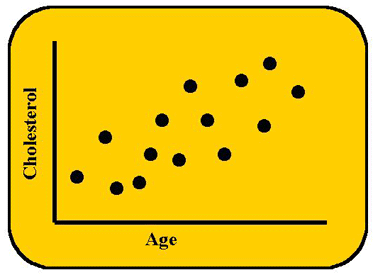
If we were to plot the relationship between cholesterol levels in the blood (on the y-axis) and a person's age (on the x-axis), we might see the results shown here. This graph is sometimes called a scattergram because the points scatter about some kind of general relationship. From the graph we can see a linear relationship - as age increases, so does the cholesterol concentration. It looks like a first-order relationship, i.e., as age increases by an amount, cholesterol increases by a predictable amount. The relationship appears so strong that knowing a person's age (predictor or independent variable) could help to infer something about his or her cholesterol level (criterion or response or dependent variable).

This scattergram demonstrates a positive relationship or positive correlation because both variables increase in the same direction. As age increases, cholesterol increases. If one variable increased while the other decreased, that would be a negative or inverse correlation and the line would decline.

Correlation Coefficient

There are a lot of other relationships that we could graph, for example, smoking and age. We would expect people from 0-16 years of age to smoke very little, from 16-65 to smoke more and from 65-80 to once again smoke less. This would not be a linear relationship, so not all relationships increase or decrease together indefinitely (or linearly). And what is more, not all relationships are strong.

Just how strongly related are two variables like age and cholesterol? That question can be answered by examining the correlation coefficient, Rho or r. The correlation coefficient represents the strength of an association and is graded from zero to 1.00. It has no units, but may be positive or negative. The table below provides a rule of thumb scale for evaluating the correlation coefficient.

Here we are talking about the Pearson Product Moment Correlation, or r, that is calculated from the following formula which predicts Y from X or y/x:

The algebraic basis of r is the z-score, and this formula represents something called the Fisher z transformation. You may remember other formulae for the calculation of the correlation coefficient, for example, another calculation is the infamous "Raw Score Formula." It takes the average student about twenty minutes to calculate a correlation by hand (with calculator) using the raw score formula. However, the computer can perform the feat in seconds. (Try the Paired-data Calculator that is part of the method validation toolkit on this website.)

When we talk about correlation this way, we are saying that Y is dependent upon X, which may suggest or imply that X causes Y. We need to be careful when we talk about causality! A correlation between two variables does not always mean a causal relationship, i.e., X causes Y to happen. There may be one or more variables intervening between X and Y, such as an unexamined variable like Z. In this example, we really cannot say that age causes cholesterol to increase. As we all know, there are many intervening variables that are important: genetics, exercise and diet to name a few. And, temporal sequence is also important when looking at causality, as X would always have to precede Y's occurrence in order to be causal. In our cholesterol example, this is not a problem. But if we wanted to say that exercise causes cholesterol to decrease, then we had better be sure that we first evaluate patients' cholesterol levels, put them on an exercise program and then measure their cholesterol levels after their participation in the program.

What if we wanted to use r to give us some idea about how closely the results of two methods compare? Presumably a high correlation between the results of two glucose methods would mean that the methods are comparable. Those who are knowledgeable about the use of statistics in method comparison studies will tell us that the correlation coefficient is not a fool-proof statistic and must be interpreted carefully. Any set of data where the points fall all on a line will give a high correlation coefficient. If a glucose method were consistently 50 mg/dl higher than another method, the results would fall on the line and the correlation coefficient would be high, even though there is a serious systematic error or inaccuracy between the methods.

Coefficient of Determination

The square of the correlation coefficient or r² is called the coefficient of determination. We will examine this r² later in regression analysis.

Simple Linear Regression or Ordinary Least Squares Prediction

If we really want a statistical test that is strong enough to attempt to predict one variable from another or to examine the relationship between two test procedures, we should use simple linear regression. Regression is more protected from the problems of indiscriminate assignment of causality because the procedure gives more information and demonstrates strength. In fact, the r that we have been talking about above is only one part of regression statistics.

Let's see how this prediction works in regression. Let us say that we have a data set for two variables X and Y. We have calculated the mean for each of these variables. Now let's say that we put all of the Y values into a container and draw one value out of that container at random. Before we look at that Y value, we first are going to guess what the number is. What value should we guess? What value would be most likely? The best guess for the value of Y would be the mean value for the Y data - the arithmetic average is always a good guess. But statisticians have worked out a better method. Another variable (X) can be used to approximate the Y. If Y is dependent upon this X, then the Y estimated this way will be closer to the true Y value than just guessing Y's mean.

Mathematical Formula for a Straight Line

In its simplest form, regression is essentially the formula for a straight line that you learned in beginning algebra. In essence, the prediction of Y from X is dependent upon the mathematical formula for a straight line. The first time you saw this formula it appeared as follows:

y = mx + b

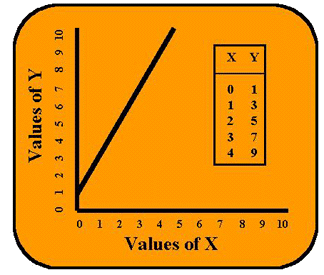
Typically in algebra, the student is asked to set up a table of x and y values, graph the points, and draw the best straight line through those points. For example, if y = 2x + 1 the table and graph would appear as shown in the accompanying figure. When x is equal to zero, y is equal to 1 because the mx term falls out [2 times 0 is 0]. In this same expression, the b-term is 1. So when x is equal to zero, y is equal to 1 [y = (2*0) + 1]. If we look at this zero point on the x-axis, the line cuts the y-axis at the number 1. We call this number the y-intercept (or constant). Now if x is any number greater than zero, the m-term or coefficient becomes important. Here m is the number 2. If we make x equal to 1, then y is 2 plus the 1 for the constant. Essentially what this m is telling us is that when x increases by a factor of one, y increases by a factor of 2. There is not 1:1 correspondence. Y is increasing twice as fast as X. And this causes the line to slant upward, so the coefficient m is called the slope of the line.

In regression, the equation for the straight line is recast as y = bx + a. This change in terminology leads to confusion. Here a is the y-intercept or constant and b is the coefficient or slope of the line. A few more words of caution about regression - as in all of statistics there are certain assumptions: the x value is a true measure, both X and Y distributions are normal, and homoscedasticity, i.e., the variance of y is the same for each value of x. Also statisticians often write the formula this way: y = bx + a + e, where e represents the error in prediction.

Interpreting the Scattergram

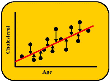
The objective in simple regression is to generate the best line between the two variables (the tabled values of X and Y), i.e., the best line that fits the data points. Regression uses a formula to calculate the slope, then another formula to calculate the y-intercept, assuming there is a straight line relationship. The best line, or fitted line, is the one that minimizes the distances of the points from the line, as shown in the accompanying figure. Since some of the distances are positive and some are negative, the distances are squared to make them additive, and the best line is one that gives lowest sum or least squares. For that reason, the regression technique will sometimes be called least squares analysis.

The fitted regression line can tell us the actual ratio for the correspondence between x and y. In the case of cholesterol vs age, we don't expect a one-to-one correspondence. However, in a comparison of cholesterol results between two different analytical methods, we would want a one-to-one correspondence, i.e., we want Method Y to give about the same results as Method X. The line of l:l correspondence should have a particular tilt to it, i.e., the line should make a 45-degree angle with the x-axis. And the formula for this line would have a slope coefficient of 1 and a y-intercept or constant term equal to zero. If our original formula, y = 2x + 1, were plotted, we would see that y increases twice as fast as x. There is not l:l correspondence, and the angle of this line is different from 45 degrees. So, by merely inspecting the line generated by least squares regression, we can make some conclusions. Lessons 13 and 14 will give us more information on the usefulness of regression.

References

1. Westgard, J. O. Basic Method Validation. Madison, WI: Westgard QC, Inc., 1999.