Guest Essay
Managing Quality in Networked Laboratories
Designing QC for a single test can be a challenge. Imagine the task of selecting the appropriate QC for more than 70 tests on multiple instruments across multiple laboratories. In this essay, Nuthar Jassam and colleagues describe how this was actually done at a network of laboratories in the UK.
Managing Quality in Networked Laboratories:
A System for Managing Quality in Networked Laboratories - statistical control rules design
Nuthar Jassam[1], Mike Bosomworth[1], Douglas thompson[1], chris lindsay[2], julian H. barth[1]
[1] Department of clinical biochemistry, the general infirmary, leeds, UK
[2] siemens healthcare diagnostics, sir william siemens square, surrey, UK
January 2012
Introduction
In most clinical laboratories, quality control is used to monitor the level of quality that is being achieved, rather than controlling a planned and defined level of quality. In several publications Westgard has presented the concept of a scientific based quality control design that optimises the error detection and minimises false rejection for an analytical process[1,2]. In order to plan appropriate control rules for an analytical process, a clear definition of the quality goal is a fundamental necessity. This should be followed by the determination of the performance characteristics (imprecision and bias) for those tests for which quality control procedures are being developed and the number of control materials to run for each test (N).
The process of IQC rule derivation starts with calculating the process capability of detecting critical random error (ΔREc) and systematic random error (ΔSEc) and makes use of operating specification charts (OPSpecs), power function graphs and method evaluation decision charts (MEDx) to define the rules that provide the highest probability of error detection (Ped) and the lowest probability of false rejection (Pfr). The process capability is also given in terms of sigma metric and defines the number of control measurements (N) for each rule or set of rules. The process capability is a term that describes the tolerance of specification to imprecision and bias within the analytical process. High capability means that the process will likely produce a result within the tolerance specification. Low capability means that the process will likely produce a result outside the tolerance specification. Westgard defines that the right quality control procedure is one that has at least 90% probability of detecting a medically important error and less than 5% probability of false rejection. Simple control rules are preferred over multirule combinations, along with the lowest number of control measurements (N) that will provide the optimal error detection [2].
The IQC design approach should ideally be derived for each individual test in a multi-test system [3]. In the USA, Westgard QC rules have been widely implemented due to the introduction of the Clinical Laboratory Improvement Amendments (CLIA) regulations which base their limits on the concept of total error (TE). However, in the UK Westgard control rules are not normally used appropriately. This is probably due to the apparent complexity of the rules deriving process, the lack of understanding of the potential benefits of this type of system or the lack of a CLIA counterpart regulatory body in the UK [4].
The perception of laboratory personnel has been that the biological variation model would be impractical in the setting of the quality specifications for clinical laboratories so this has limited the implementation of these types of quality specifications. We recently reviewed the quality system for our network and derived quality specifications based on the biological variation model [5]. We compared our system performance characteristics in term of imprecision and bias against allowable imprecision and bias derived from the biological variation. This provided us with the first evidence of the practicality of this approach in a network of laboratories. We demonstrated that in a network of laboratories analytical variability between instruments of the same type does exist. Controlling variability requires a system that detects analytical error at the analytical stage. In this study we apply a well described scientific approach to control analytical variability within our network of laboratories. The concept was based on the application of analyte/analyser specific quality control rules (Westgard rules). The design of these rules takes into account the performance of a method and its quality analytical goal. The objective is to maximise the ability of our quality control process to detect the clinically relevant analytical error and control the across site analytical variability.
Method
Analytical system: The analytical platforms consist of nine general chemistry analysers (Advia 1200, 1800, 1650 and 2400) and seven immunoassay analysers, all Centaur XP. These analysers were located on four geographically distant laboratories. All analysers were from a single manufacturer (Siemens Healthcare Solutions, Camberley, UK). All reagents (except 4 methods) were also from Siemens. The Internal Quality Control materials (IQC) were from Bio-Rad Laboratories, UK. The quality control procedure initially in use across all the network laboratories was 12s (Mean ± 2SD). Two control materials were measured per run (N=2). The frequencies for the IQC measurement for Advia were hourly and for the immunoassay were three times a day through the daily operation.
Quality control planning
Quality specifications: The clinical requirements for quality were defined for all 71 tests measured in the core biochemistry laboratories. These tests include general blood and urine chemistries, endocrinology, therapeutic drug monitoring, tumour markers and cardiac troponin. The clinical requirements were defined at concentrations close to the clinical decision limit for each test and were given in terms of total allowable error (TEallowable), allowable imprecision (CVallowable) and allowable bias (Ballowable). The mechanism of the process for biological variation derived specification has been described [5].
Performance characteristics of current assays: Estimates of stable analytical imprecision (CVanalytical) were calculated for each of the 71 analytes from the average CV over a 6 month period and estimates of bias were calculated from EQA return data over the previous year. The mean bias over this time was calculated as a percentage difference of the method group mean. (BM = (result – method group mean)/method group mean * 100).
Assessing system capability: The size of critical systematic error (ΔSEc) and critical random (ΔREc) that need to be detected to maintain the clinical requirements for quality were calculated by EZ Rules® 3 software package (www.westgard.com) as follows:
ΔSEc = [(TEallowable – BM) / CVA]-1.65
ΔREc = (TEallowable – BM) / 1.96 CVA
Sigma metric also indicates the system capability and it is calculated by the EZ Rules® 3 software as:
σ = [(TEallowable – BM) / CVA]
where TEallowable is the allowable total error requirement for the test in question, analytical imprecision and analytical bias are the estimates of stable observed CVA and BM for the test in question. The biological TEallowable, biological CVallowable and biological Ballowable were entered in the EZ Rules® 3 software package under biological total error mode. The TE value was entered under the analytical total error mode for all the analytes with other forms of quality specifications. The observed CVA and BM for each test and the clinical decision limit data for each test were also fed into the EZ Rules® 3 software. The optimal QC rules procedure that provides the best error detection and lowest false detection was selected automatically by the software. The probability of Ped and Pfr for the 12s rules for all studied tests was selected manually.
Results
Quality specifications
Quality specifications for our network were derived from three models; (1) the biological variation based model; the three levels model (TLM) (46 analytes)[6], (2) the pharmacokinetic model as described by Fraser[7] (9 therapeutic drugs) , (3) a mixed quality specification model based on expert opinion and external quality control specifications, which included 16 analytes. Three analytes did not fit with any form of specification due to poor performance. Figure 1 shows the distribution of the 71 studied analytes across the three types of quality specifications and it also shows the allocation of the 46 analytes with biological variation derived TE allowable to each level of the TLM model.
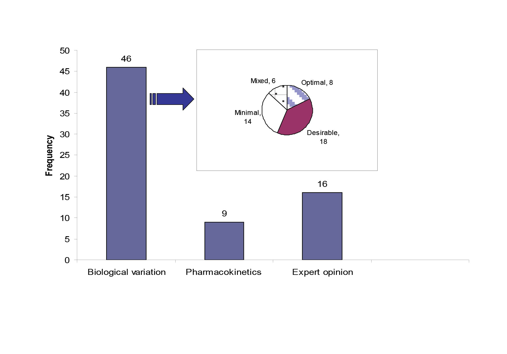
Figure 1: The source of quality specifications for the 71 analytes measured within the core biochemistry laboratories.
The pie chart shows the quality specification allocation for the analytes with TE derived from the TLM. The mixed category for analytes has the bias and CV limits selected from different levels in the TLM.
Fourteen analytes had TEallowable allocated to the minimal level. Seven out of fourteen were allocated to this level of performance due to unsatisfactory current analytical performance. The other seven were allocated to the minimal level because allocation to the desirable level wouldn’t result in an improvement in quality. The 95% dispersion around the clinically relevant decision point showed that there was no significant difference between the desirable and the minimal CV levels (Table 1).
Table 1: Detailed performance of the 14 analytes that were allocated to the Minimal level of TE specification.
Highlighted are 7 analytes where the CVminimal would produce either the same/or not clinically significant variation range around the selected concentration as the CVdesirable
| Analyte | Cut off | TE |
Variation around thecut off atCVanalytical |
Variation aroundthe cut off atCVOptimal |
Variation aroundthe cut off atCVDesirable |
Variation aroundthe cut off atCVMinimal |
Sigma-metric |
| ALP | 300 iu/L | 52 iu/L | 258-342 | 262-338 | 258-342 | 253-347 | 8.0 |
| GGT | 50iu/L | 16.6 iu/L | 35-65 | 36-64 | 35-65 | 33-67 | 4.8 |
| HDL-cholesterol | 1mmol/L | 0.13 mmo/L | 0.9-1.1 | 0.9-1.1 | 0.8-1.2 | 0.8-1.2 | 4.7 |
| LDH | 430 iu/L | 74 iu/L | 355-505 | 355-505 | 349-511 | 339-521 | 6.0 |
| K | 4 mmol/L | 0.35 mmol/L | 3.6-4.4 | 3.6-4.4 | 3.6-4.4 | 3.5-4.5 | 3.4 |
| AFP | 5 iu/L | 1.6 iu/L | 4-6 | 4.0-6.0 | 4.0-6.0 | 4.0-6.0 | 3.6 |
| Ca 125 | 10 ku/L | 3.5ku/L | 7-13 | 7.0-13 | 7.0-13 | 7.0-13 | 4.8 |
| CEA | 10 g/L | 4 g/L | 7-13 | 7.0-13 | 7.0-13 | 7.0-13 | 4.8 |
| FSH | 5 iu/L | 1.3 iu/L | 3.8-6.2 | 4.0-6.0 | 3.9-6.1 | 3.8-6.2 | 3.3 |
| LH | 5 iu/L | 1.5 | 3.3-6.7 | 3.5-6.5 | 3.4-6.6 | 3.2-6.8 | 4.9 |
| Total protein | 70g/L | 3.5 g/L | 66-74 | 66-74 | 66 -74 | 65-75 | 2.4 |
| Testosterone-M | 10 nmol/L | 2.6 | 7.2-12.8 | 8.1-11.9 | 8.0-10.0 | 7.7-12.3 | 1.8 |
| Testosterone-F | 2.5nmo/L | 0.65 | 1.8-3.2 | 2.0-3.0 | 2.0-3.0 | 1.9-3.1 | 1.8 |
| TT3 | 3 nmol/L | 0.75 nmol/L | 2.1-3.9 | 2.5-3.5 | 2.4-3.6 | 2.4-3.6 | 1.7 |
Westgard QC rules
Analyte specific control rules were derived for 68/71 tests performed in the core biochemistry laboratories in the network. A total of 35/71 (50%) analytes were controlled by a single rule only. Thirty of these were for analytes with TE based on biological variation. The new rules were more relaxed than those originally used (12S) in the laboratories (32 analytes with 12.5S or 13S or 13.5S at N= 2 and 3 analytes with a 12.5S and N=4). These analytes were alkaline phosphatase (ALP), alanine transferase (ALT), amylase, gamma glutamyl transferase (GGT), creatine kinase (CK), C-reactive protein (CRP), cholesterol, HDL-cholesterol, creatinine, triglycerides, conjugated bilirbin, total bilirubin, lactate dehydrogenase (LDH), iron, lactate, uric acid, urea, Ca-19-9 and Ca-125, troponin (TnI), prostate specific antigen (PSA), salicylate and all tests for urine chemistry except urine albumin.
Eight out of 71 analytes had multi-rules 13S/22S/ R4S/ 41S at N=4, these were albumin, calcium, chloride, potassium, lithium, prolactin, thyroid anti-peroxidase (TPO) and thyroid stimulating hormone (TSH).
Maximum control rules 13S/22S/ R4S/ 41S / 8X at N=4 were required to control the performance of 11/71 analytes. These analytes were glucose, bicarbonate, magnesium, sodium, total protein, progesterone, testosterone, total triiodothyronine (TT3), total thyroxine (TT4), carbamazipne, and urine albumin.
14/71 analytes required different controls rules on different sites. These analytes were conjugated bilirubin, cholesterol, HDL-cholesterol, uric acid, α- feto protein (AFP), carcino-embryonic antigen (CEA), cortisol, luteinising hormone (LH), follicle stimulating hormone (FSH), human chorionic gonadotrophin (hCG), parathyroid hormone (PTH), paracetamol, theophylline, urine protein and urine uric acid. The requirement for different control rules was due to the difference in observed bias and imprecision across sites e.g. cholesterol; this analyte required 12.5S, N=2 on three sites and 13.5S, N=2 on one site. Serum uric acid required a single rule to control its performance on three sites and maximum rules 13S/22S/ R4S/ 41S /8X at N=4 on one site.
Three analytes had unacceptable performance and were impossible to control by any control rule; these were free thyroxine (fT4), digoxin and oestradiol.
System capabilities in terms of sigma
Using the biological variation derived TE specifications, we found that 50% (23) analytes perform at a level of 5 sigma or higher, 20% (9) analytes performed at sigma varying between 4 and 5, 20% (9) analytes performed at 3-4 sigma and 10% (5 analytes) performed at sigma less than 3. Figure 2 gives the analytical performance of the biological variation based quality specification analytes in terms of sigma (σ).
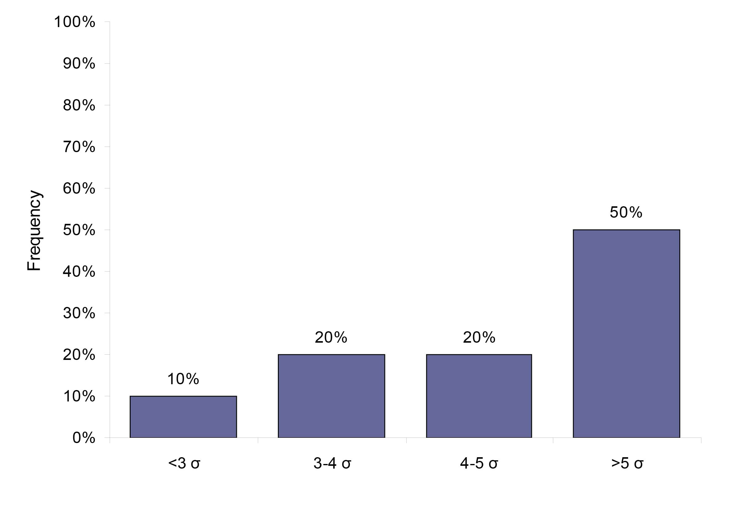
Figure 2: The system capabilities given in sigma for the 46 analytes that have a quality specification based on biological variation.
Comparison of the new and old quality system
The probability of false rejection was set to be maximally at 5% for the new rules selection. The 12s rule usually has a false rejection of 9%. Table 2 shows ped and pfr with the new rules and with the 12s rule for the general chemistry only.
Discussion
Until recently we had used a simple Westgard rule system 12s (mean ± 2 SD) for controlling analysers on each site across our multi-site laboratory network. As described previously this was not satisfactory for the control of analysers across the network[5]. Furthermore, this rule has Pfr of 9% at 2 control measurements . This high false rejection rate would render this rule a major waste of laboratory resources due to repeat analysis of controls, and patients’ samples resulting in an increase in the cost of the analytical process and a waste of time and effort. If we considered the number of analytes measured and the volume of testing performed on a daily basis in our network of laboratories, which exceeds 20,000 tests per day, one would assume this could be a significant waste of the laboratory budget.
This type of waste can be avoided by designing a quality control procedure that is based on the quality goal required clinically and the performance characteristics of each test/analyser[10]. Therefore, the laboratory's efforts would be focused on the analytes that require the maximum control. The ideal IQC design should be derived for each individual test in a multi-test system, selecting where possible the combination of the highest Ped and the lowest Pfr [3]. In this study, the quality control rules were selected at the Pfr has been set at a maximum of 5%. This has resulted in a cumulative reduction in the Pfr by more than 50% (Table 2).
| Analyte | New Rules | Old Rule: 12s | ||
| Systematic error | Random error | Systematic error | Random error | |
| Ped/Pfr | Ped/Pfr | Ped/Pfr | Ped/Pfr | |
| Albumin | 65/3 | 61/3 | 66/9 | 48/9 |
| Amylase | 97/3 | 67/3 | 100/9 | 77/9 |
| ALP | 89/0 | 61/0 | 100/9 | 83/9 |
| ALT | 96/3 | 66/2 | 99/9 | 75/9 |
| Bicarbonate | 0/3 | 0/4 | 0/9 | 0/9 |
| Calcium | 82/3 | 73/3 | 79/9 | 60/9 |
| CRP | 98/0 | 61/2 | 100/9 | 83/9 |
| Conjugated bilirubin | 98/0 | 62/0 | 100/9 | 80/9 |
| GGT | 93/3 | 64/2 | 99/9 | 74/9 |
| Cholesterol | 95/3 | 65/2 | 95/1 | 65/2 |
| Creatine kinase | 98/0 | 62/0 | 100/9 | 80/09 |
| Chloride | 91/4 | 74/4 | 87/9 | 61/9 |
| Glucose | 27/3 | 30/4 | 24/9 | 30/9 |
| HDL-cholesterol | 90/3 | 61/2 | 100/9 | 76/9 |
| Iron | 89/0 | 61/0 | 100/9 | 81/9 |
| LDH | 89/0 | 55/2 | 100/9 | 81/9 |
| Lactate | 89/0 | 61/0 | 100/9 | 83/9 |
| Potassium | 62/3 | 60/3 | 64/9 | 47/9 |
| Magnesium | 23/3 | 28/4 | 22/9 | 28/9 |
| Sodium | 23/3 | 28/4 | 16/9 | 11/9 |
| Phosphate | 83/3 | 68/3 | 85/9 | 68/9 |
| Total bilirubin | 98/0 | 61/0 | 100/9 | 80/9 |
| Total protein | 22/2 | 27/2 | 21/9 | 0/9 |
| Triglycerides | 97/3 | 67/2 | 100/9 | 77/9 |
| Uric acid | 89/0 | 61/0 | 89/9 | 62/9 |
| Urea | 97/3 | 67/2 | 100/9 | 77/9 |
Table 2: The probability of error of detection (PED) and the probability of false rejection (PFR) of the new quality control rules in comparison to the OLD QC RULES (12s rule).
The ALP and total protein examples are highlighted. ALP: the QC rules selected for this analyte will give the probability of systematic error detection of 89% and random error detection of 61%. The false rejection for these rules is zero. The current rule 12s has higher error detection but almost one run in ten has a false error. For total protein, both the new rules and the current rule have poor error detection. However, the false rejection in the current rule is over 40% ( 9/21). This means that over 40 times out of 100 runs the analyser would have been stopped for a false error flag.
It was also found that 19 analytes required multi-rules or maximum rules to control the analytical process required to satisfy the quality goal. This shows that the initial 12s rule alone has not been efficient enough to control the performance of these analytes, hence the variability in analytical performance between sites. Furthermore, 14 analytes required different quality control rules on different sites, or on different instruments within the same site. As the same analyte has the same TE across all sites, the difference in the quality control rules required stems from a difference in the performance indicators of these analytes, which as described previously can be ascribed to varying levels of hardware deterioration of the instruments on different sites. This can be due to different workloads or an inherent difference in the design of those instruments.
The new quality control rules rely on a scientific approach, taking into account the quality goal and the observed performance of an analytical method. For example, if the analytical process is more precise than medically required (e.g. iron, TE= optimal, σ= 7.5) the quality control process can be relaxed and would only need one rule such as 13s to achieve the required quality goal. Controlling these analytes with 12s or multi-rules would have resulted in a waste of resources. However, assays with unsatisfactory performance (low system capability or low sigma) may require the maximum control rules to achieve the desired goal. Our data showed that for 50% of total analytes measured in the core biochemistry a more relaxed rule than the initial rule in use could be used. This shows that this control rule design provides a cost effective model because the decrease in the cost of controlling the analytes with more relaxed control rules is transferred to those tests that require a higher degree of control.
World class quality is generally recognised as a 6 sigma process (3.4 defects per million on the sigma short-term scale). The 3 sigma performance (66,807 defect per million on the short-term scale) represents the minimum standard and defines the region of unacceptable performance . In the clinical laboratories improving processes to achieve a performance above 5 sigma (233 defects per million on the sigma short-term scale) is of little advantage and can be costly[9]. Performance at 4 sigma (6,210 defect per million on the sigma short-term scale) is considered satisfactory for the clinical laboratory if the process is adequately controlled [9]. Using the biological variation based TE resulted in achieving performance of 4-6 sigma for 70% of the analytes. However, it is important to recognise that the size of critical error (systematic/random) or sigma index depends on the allowable TE and the performance of the measurement system. A smaller total error or poor CV and bias would result in a small sigma or critical error. Biological variation based quality specifications represent a narrow form of quality specifications, which means that we have to detect a smaller but clinically relevant change in the analytical process. In this case, achieving a smaller sigma but a narrower quality requirement is better [10]. Our data showed that 30% of the studied analytes had a performance consistent with a poor sigma (σ ≤ 4), however, most of these analytes had a CV within the biological variation for all the sites. For example, glucose had an average analytical CV ≤ the allowable CV (2.9% (desirable level)) on all sites. Given that the TEallowable is 6.9%, a CV of 2.9% would result in performance of 2.4σ, whereas improving the analytical performance to achieve a CV of 1.4% (optimal CV), which meet 5σ performance remains a goal for this analyte.
On the other hand, for some analytes that were allocated to the minimal level due to current unsatisfactory performance, achieving 5 sigma would be challenging without an improvement in the method technology and formulation.
In our study, we presented a central quality system that enables the identification of poor performance in the analytical process in a retrospective manner [5]. The system was based on quality specifications derived from biological variation data and software that enabled the application of common specifications and across laboratory analytical performance comparison. In this paper, we have added the last dimension to this system. This was based on deriving analyte specific quality control rules that maximise the detection of analytical error during the analytical stage, and helps to maintain a stable analytical performance.
As far as we know this is the first attempt to test the practicality of quality specifications based on biological variation to control the analytical performance across a multi-site network. We have demonstrated that the biological variation model is a practical model with which to derive quality control specifications that are related to the clinical requirements of a test and we have designed quality control rules to maintain the stability of the analytical process
Appendix
Biological variation based quality specification: Glucose
The formula for calculating the dispersion that encompasses 95% of values is:
CVTotal = ± 1.96 (CVa2+CVI2)1/2
SDTotal = CVTotal × test concentration / 100
95% dispersion interval = test concentration ± SDTotal
The ‘current' data field represents the worst imprecision over a 6 month period across all the analysers in the network.
The CVI values for glucose, 5.7% [12 ].
The effect of imprecision at the three performance levels around a glucose concentration of 7.0 mmol/L.
| Performance level | CV% | %CVTotal | 95% dispersion interval at glucose of 7.0 mmol/L |
| Optimal | 1.4 | 11.5 | 6.2 - 7.8> |
| Desirable | 2.9 | 12.5 | 6.1 - 7.9 |
| Minimal | 4.3 | 14.0 | 6.0 - 8.0 |
| Current | 2.9 | 12.5 | 6.1 - 7.9 |
Glucose is reported to one digit after the decimal point through the whole range. Our current performance lies within the desirable level. However, the optimal level gave the least dispersion interval. A cut off of around 7.0 mmol/L glucose is used diagnostically, hence we believe that the optimal performance level is the ideal target to achieve clinical decision making.
Total error estimation based on expert opinion: Prolactin
Biological variation data for prolactin (PRL) is not available. TE was estimated on the basis of the tolerance around a clinically relevant cut off value and current performance. The cut off for PRL was selected as the upper limit for monomeric PRL reference range (438 mu/L) [13].
Allowable CV= 10% (based on an average of 6 months performance).
Allowable bias: 10% (The 75 quartile of the method group in NEQAS scheme).
Allowable TE= Bias + 1.65CV
Allowable TE= 26.5%
Quality specifications based on pharmacokinetics theory: phenytoin
Some quantities that are measured in clinical biochemistry do not exhibit biological variability such as drugs. For these analytes, Fraser et al. derived a formula to calculate the desirable analytical goal for precision based on the fundamental pharmacokinetics theory [14]. Phenytoin is an anti-convulsant drug with a half life in chronic administration of between 6 and 24 hours. [15].
| Half life | %CV analytical < 1/4 x [(2T/t - 1)/ ( 2T/t + 1) x 100 |
| 6 hours | 22% |
| 24 hours | 8.3% |
| Current | 7 % |
In premature babies, phenytoin has a long half life due to the immaturity of the liver. The longest half life was used to derive a quality specification for this analyte, because it can deliver the most stringent analytical goal. Therefore the desirable CV is 8.3%.
Method bias= 10% (estimated from the External Quality Assurance Scheme).
TE allowable= B+1.65 CV
= 23.6%
References
- Westgard JO. A method evaluation decision chart (MEDx chart) for judging method performance. Clin Lab Sci 1995; 8: 277-283.
- Westgard JO. Internal quality control: planning and implementation strategies. Ann Clin Biochem 2003; 40: 93-611.
- Westgard QC, Inc,. EZ Rules ® 3 automatic selection of statistical control rules for laboratory tests. Madison, WI: Westgard QC. Inc,. 2005.
- Housley D, Kearney E, English E, et al. Audit of internal quality control practice and processes in the south-east of England and suggested regional standards. Ann Clin Biochem 2008; 45: 135-139.
- Jassam N, Lindsay C, Harrison K et al. A system for managing analytical quality in networked laboratories: the implementation. [ in preparation]
- Fraser CG, Hyltoft Petersen P, Libeer JC, Ricos C. Proposal for setting generally applicable quality goals solely based on biology. Ann Clin Biochem 1997; 34: 8-12.
- Fraser CG. Desirable standards of performance for therapeutic drug monitoring. Clin Chem 1987; 33: 387-389.
- Westgard lesson. Six sigma quality management and Desirable laboratory precision. www.westgard.com/essay35.htm (accessed 2/12/2009).
- Westgard JO. Six sigma quality design and control: desirable precision and requisite QC for laboratory measurement process. Madison, WI: Westgard QC, inc., 2001.
- Westgard lesson. www.westgard.com/a-six-sigma-design-tool.htm (accessed 2/12/2009).
- Campbell BG. Evaluation of two types of medically significant error limits and quality control procedures on a multichannel analyser. Arch Pathol Lab Med 1989; 113:834-7.
- Ricós C, Alvarez V, Cava F, et al. Desirable quality specifications for total error, imprecision, and bias, derived from biological variation. www.westgard.com/biodatabase1.htm (accessed on 6/09/2009).
- Jassam NF, Paterson A, Lippiatt C, Barth J. Macroprolactin on the adiva centaur: experience with 409 patients over a three-year period. Ann Clin Biochem 2009; 46:501-504.
- Fraser CG. Desirable standards of performance for therapeutic drug monitoring. Clin Chem 1987; 33: 387-389.
- Mike Hallworth and Ian Watson. Ed. Therapeutic drug monitoring and laboratory medicine. ACB Venture Publications 2008.