Quality Requirements and Standards

Part 2 in a discussion of the state of debate around quality, performance specifications, measurement uncertainty, and the meaning of life.

Perspectives on Analytical Quality Management

Part 2. Setting Control Limits on Control Charts

James O. Westgard, PhD
August 2022

Everybody knows it's coming apart
Take one last look at this Sacred Heart
Before it blows
And everybody knows
Leonard Cohen – Everybody Knows

This is an extension of the discussion of new metrologist recommendations to set control limits on control charts using an acceptance range based on Analytical Performance Specifications for Measurement Uncertainty, i.e., a 95% range expressed as 2*APSu, where APSu represents the allowable standard measurement uncertainty [1]. We consider that advice to be wrong [2] and instead recommend following the CLSI C24-Ed4 “roadmap” for planning SQC strategies [3]. Metrologists oppose that approach because it illustrates the use of a quality goal for Total Analytical Error to guide the selection of appropriate control rules, numbers of control measurements, and frequency of QC events [4].

[Quick Recap: Part I in this series discussed the mistaken notion that an objection to a TEa goal-setting model discredits the TAE model for assessing the method performance and planning SQC strategies. We pointed out there is confusion between two different models – a TAE model for quality assessment/control and a TEa model for goal setting. The TAE model is part of the Six Sigma Quality Management framework that we recommend. The TEa goal-setting model is part of the database on biologic variation and analytical performance specifications that is supported and maintained by the European Federation of Laboratory Medicine (EFLM).]

This second discussion considers a fundamental principle of SQC for setting control limits on control charts. Everybody knows the accepted practice is to calculate control limits based on the mean (set as TV) and SD observed for each individual method in the laboratory. But this long-standing principle will be blown away by the metrologists’ re-design of IQC.

The Two Component IQC Proposal

From Braga et al [1, Abstract, page 291]: “…the internal quality control (IQC) program should be redesigned to permit IVD traceability surveillance through the verification by medical laboratories that control materials, provided by the manufacturer as a part of measuring systems, are in clinically suitable validation range (IQC component I). Separately, laboratories should also monitor the reliability of employed IVD measuring systems through the IQC component II, devoted to estimation of MU due to random effects and to obtaining MU of provided results, in order to apply prompt corrective actions if the performance is worsening when compared to appropriate analytical specifications, thus jeopardizing the clinical validity of test results.”

It should go without saying that a proposal to double the work required of a laboratory is likely to meet with strenuous objections.  Given that it takes several months to estimate MU with Component II, it’s not clear how it can be used to “apply prompt corrective actions.” Also, if MU is estimated only once every six months, it will have limited capability to “monitor the reliability of employed IVC measuring systems.” However, our interest and priority here is to consider the recommended re-design of Component I, the traditional QC, particularly the idea of imposing limits on control charts using an acceptability range derived from the Analytical Performance Specification for Measurement Uncertainty.

Component I Control Limits - One MU to rule them all?

From Braga et al [1, page 296]: “… the acceptability range for QC component I should correspond to the APS for MU derived according to the appropriate Milan model and its should be set based on unbiased target value of the material obtained by the manufacturer as the mean of replicate measurements on the same measuring system optimally calibrated to the selected reference…”

The recommendation here is to use fixed clinical control limits based on the quality goal or APS for MU, as derived from biologic variability and the EFLM biological variation database. In other words, the control limits (TV ± 2*APSu) are the same for all laboratories that follows the EFLM guidance, regardless of the actual performance of a particular laboratory. This “one-size fits all” approach is a direct contradiction of the “good laboratory practices” for statistical QC summarized by the CLSI C24-Ed4 [3]. Common sense tells us that all laboratories are not identical in performance the world over. The desire to impose the same rule across the globe is tantalizing, but reality must be acknowledged.

From CLSI C24-Ed4 [3, page 27, Section 5.3]: “A target value and SD for a particular control material are established by the laboratory. The mean, used as the target value, and the SD of results are established by repeated measurements of the QC materials by the measurement procedure used by the laboratory. Control limits are then calculated from the target value and SD observed in the laboratory when the measurement procedure is operating in stable condition. When control materials are accompanied by a product insert with assigned values provided by the manufacturer, these insert values should be used only as guides and not as a replacement for target values and SDs established by the laboratory.”

This contradiction is recognized by the authors, who explicitly disregard the CLSI guidance:

From Panteghini [4]: “…the fundamental principle of CLSI C24-Ed4 guideline is that each laboratory should characterize its own performance, using its experimental mean and SD in calculation of control limits. This make however impossible to establish if the individual measuring system performance is properly unbiased…”

HbA1c Example

APSu for HbA1c is 3.0%, according to recommendations by these authors [5], so the acceptability range of ± 2*APSu would be TV ± 6.0%.

• A method having stable imprecision of 1.0% and bias of 0.0% demonstrates 6-Sigma performance [Sigma = (2*APSu-%|Bias|)/%CV or (6.0%-0.0%)/1.0%] and the MU acceptability range provides a 6s control range (6.0%/1.0%).
• A method having stable imprecision of 1.5% and bias of 0.0% demonstrates 4-Sigma performance, which should require more intensive QC.
• A method having a CV of 2.0% and bias of 0.0% would provide only 3-Sigma performance, which according to industrial guidelines borders on being unacceptable for routine production.

How can a single “acceptability range” of TV ± 6.0% provide appropriate QC for methods that vary from 3.0 to 6.0 Sigma?  From experience, our QC “rules of thumb” are that a 6-Sigma method can be adequately controlled using a 1:3s rule and N of 2; a 4-Sigma method requires a multirule QC procedure with an N of 4; and a 3-Sigma method would require so much QC that it might be too expensive and impractical to operate in healthcare laboratories. With Westgard Sigma Rules, you can adjust QC for the performance of the method. The metrologist approach has no flexibility, no customization, no deviation allowed.

Graphical assessment of performance of a clinical control limit

For the situation where there is only one control measurement, a simple graphical assessment is revealing. Consider again our HbA1c method with the quality requirement being defined as 2*APSu or 6.0% in Figure 1.

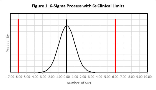
Figure 1 shows the error distribution for a method having a bias of 0.0 and an SD (or CV) of 1.0. With a bias of 0.0, the distribution is centered on 0.0 on the x-axis and mostly contained within ± 3 SDs. The clinical limits of ± 2*APSu are shown as the solid red lines at ± 6.0 SDs. This would be considered an example of a method with “world class quality.”

Figure 2 shows this same situation (6-Sigma quality) where the original error distribution (indicated by the dashed line) has shifted by an amount equivalent to 6s (solid line), which is the size of the supposed Clinical Control Limit. As shown by the amount of the error distribution that exceeds the Clinical Control Limit, this medically important error will be detected only 50% of the time. That of course means that the other 50% of the time this medically important error will not be detected, even though the control limits are fixed clinical limits of ± 6s. Thus it should be readily apparent that so-called “clinical control limits” will not provide a high confidence or high probability of detecting medically important errors.

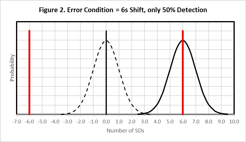
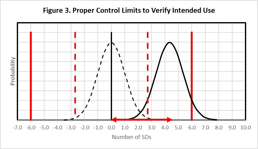
 Figure 3 shows that to achieve the appropriate error detection and reduce (to 5%) the number of results that might exceed the clinical requirement, it would be necessary for the error distribution to be located to the left, equivalent to a 4.35s shift as shown by the horizontal red error bar on the bottom x-axis, then set the control limits even closer to the original distribution, as shown by the dashed red vertical lines, so that at least 90% of that distribution exceeds the statistical control limit. The systematic shift must be limited to 4.35s and the control limits set close to 3.0s to provide adequate error detection when method precision is 1.0%, bias is 0.0%, and 2*APSu is 6.0%. Thus, to achieve high detection of medically important errors, it is necessary to set the control limit such that almost the entire shifted distribution exceeds the control limit while at the same time allowing only 5% of the shifted distribution to exceed the quality requirement.

What’s the point?

Setting proper control limits on a QC chart is not so simple as drawing fixed “acceptability limits” such as TV ± 2*APSu directly on control charts. As demonstrated here, such limits will not provide sufficient detection of medically important errors. Instead, a structured QC planning process should be implemented to identify appropriate control rules, numbers of control measurements, and frequency of QC events, taking into account the quality required for the intended use of the test, the precision and bias of the method, and the rejection characteristics of statistical QC rules. The key to a quantitative planning process is the use of power curves that describe the probability for rejection as a function of the size of systematic errors, or alternatively, as a function of the Sigma-metric of the method. CLSI C24-Ed4 describes a “roadmap” for planning risk-based SQC strategies that also consider patient risk due to reporting of erroneous test results. Graphical QC planning tools are available to support such a planning process. This approach will be discussed in more detail in parts 3 and 4 of this series.

References

1. Braga F, Pasqualetti S, Aloisio E, Panteghini M. The internal quality control in the traceability era. Clin Chem Lab Med 2021;59:291-300.
2. Westgard JO, Bayat H, Westgard SA. How to evaluate fixed clinical QC limits vs. risk-based SQC strategies. LTE: Clin Chem Lab Med 2022; https://doi.org/10.1515/cclm-2022-0539.
3. CLSI C24-Ed4. Statistical Quality Control for Quantitative Measurement Procedures: Principles and Definitions. 4th ed. Clinical and Laboratory Standards Institute, 9950 West Valley Road, Suite 2500, Wayne PA, 2016.
4. Panteghini M. Reply to Westgard et al.: ‘Keep your eyes wide… as the present now will later be past.’ LTE: Clin Chem Lab Med 2022; https://doi.org/10.1515/cclm-2022-0557.
5. Braga F, Panteghini M. Performance specifications for measurement uncertainty of common biochemical measurands according to Milan models. Clin Chem Lab Med 2021;59:1362-1368.