Z-Stats / Basic Statistics
Z-9: Truth or Consequences for a Statistical Test of Significance
How much power does a statistical test have? What do the results of a statistical test mean? Dr. Zady weighs in on this matter and gives you guidance on how you should weigh the results of your tests.
EdD, Assistant Professor
Clinical Laboratory Science Program, University of Louisville
Louisville, Kentucky
- Truth table and classification errors
- Consequences and performance characteristics
- Effect of experimental factors
- References
Lessons 6, 7, and 8 examined hypothesis testing using the t-test as the example test of significance. In this lesson, we are going to look more closely at the correctness of a statistical test and it's "power" to detect changes. If you have a good understanding of the performance characteristics of a statistical test of significance, you will be in a better position to properly design experiments and correctly interpret experimental results.
Truth table and classification errors
In a statistical test of significance, the result is either to accept or reject the null hypothesis, Ho, which, in the case of a t-test, states there is no difference between the mean of a control group and experimental group. In reality, there either is a difference in the test groups or there isn't. Ideally, the test of significance should reject Ho whenever there is a difference and accept Ho when none exists. However, we know the world is seldom perfect and the actual behavior of a test may be less than ideal.
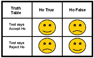 Behavior can be described by a "truth table", in this case a 2 by 2 classification table that shows all the possible outcomes. As illustrated here, the "happy" faces show the desired behavior when Ho is accepted AND there is no difference between means (a true acceptance, upper left corner of table) and when Ho is rejected AND a difference exists (a true rejection, lower right). The "unhappy" faces show our disappointment with the statistical test when it accepts a situation as "no difference between means" AND a difference really does exist (a false acceptance, upper right corner) and when rejects the two means as being the same AND there is no real difference (a false rejection, lower left).
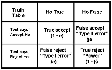 A more scientific presentation of the truth table is shown here, which identifies the possible classifications as true accept, false accept, false reject, and true reject. In statistical terminology, false reject results are called "Type I errors" and symbolized as a. In experimental design, these are common because we often set a at 0.05 and, therefore, expect a false rejection 5% of the time. The other type of error, "Type II errors," are false acceptances, which are given the symbol b. These are critical because of our interest in achieving a high rate of true rejection results, which are equal to 1 - b, also called "statistical power" or just "power". We usually want to achieve statistical power of 90 to 95%, which means b can only be 5 to 10%.
We sometimes call this truth table the "confusion matrix" [1] because of the difficulty it poses for students. There are many new concepts - true accept, false accept, false reject, true reject - as well as many new terms - Type I error, Type II error, a, b, and power. The happy face table should help you keep the concepts straight. Unfortunately, you'll have to learn the statistical terminology by rote as there's no real logic for calling one error Type I or an alpha error and another Type II or a beta error.
Consequences and performance characteristics
To understand the importance of the characteristics identified in the truth table, we need to consider the consequences of using a statistical test to compare an experimental group with a control group. We'll focus on two different situations - the first where there is no overlap between the control group and the experimental group, and the second where the two groups do overlap.
Type I and Type II errors
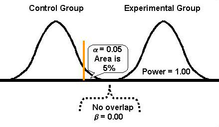 If the expected distributions for the means of the control and experimental groups are completely separated, as shown in this figure, then there shouldn't be any misclassification errors. Type I and Type II errors would not exist, i.e., a and b are 0.00 and there shouldn't be any false rejections or false acceptances of Ho. Because b is 0.00, statistical power should be 1.00 (1-b = 1.00), which means the difference between the two groups will always be detected. These values (a=0.00, b=0.00, power=1.00) represent the ideal performance characteristics for a statistical test of significance.
In practice, we usually select the alpha level to be suitably low, often a probability of 0.05, which means there would be only a 5% chance of falsely rejecting the null hypothesis and concluding that a difference exists when in fact there is no difference (Type I error). Observe the vertical line or gate that corresponds to an alpha level of 0.05 and cuts off 5% of the tail of the control distribution. Even though there is a 5% chance for a Type I error, there still shouldn't be any Type II errors where we would accept a false null hypothesis. Again, these curves are distinct, therefore, power is at its maximum.
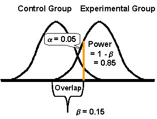 If the distributions overlap, as shown here, then the performance characteristics of the statistical test will depend on the amount of the overlap. Type I and II errors will not be zero and power will be less than ideal. The choice of a will affect the number of Type II or beta-errors and the statistical power of the test. In the example here, the alpha level is again set at 0.05. The probability of a Type II or beta-error is given as 0.15 or the area of overlap between the two curves, which leaves the statistical power as 0.85, i.e., the area of non-overlap. This indicates there is only an 85% chance of detecting the difference between the groups, or there is a 15% chance that the difference between groups may go undetected.
Statistical power
To understand power, look at the distribution of the experimental group. See how much of the area of that distribution is beyond the vertical line corresponding to the 0.05 alpha level. In the first figure, the entire distribution is to the right of the vertical line, therefore power is maximum. In the second figure, only part of the distribution is to the right of the vertical line. Obviously, power is reduced when the difference between the two groups is reduced.
Power shows the capability of an experiment to detect a difference of a certain magnitude. The larger the difference between the experimental group and the control group, the less overlap between the two groups, and the more power for detecting the difference. The greater the overlap, the lower the power. In effect, large differences will be easy to detect and small differences will be difficult to detect.
Effect of experimental factors
An understanding of these performance characteristics is important for both planning an experiment and for interpreting the results of an experiment. You are in control of some important factors when you design an experiment. Knowledge of their effects will help you to plan a better experiment. If you aren't in control of the experimental design, then you need to be aware of the potential effects of these factors when interpreting experimental results.
Choice of alpha level
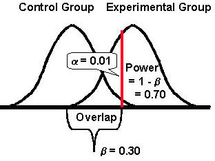 The most common error in statistical testing is Type I where a true Ho is rejected. It seems that researchers are at times overly zealous in their desire to reject the null hypothesis and to prove their point. One way to protect against Type I error is to reduce the alpha level to say 0.01, as illustrated here. With an alpha level of 0.01, there will be only a 1% chance of rejecting a true Ho. The change in alpha will also effect the Type II error, in the opposite direction. Decreasing alpha from 0.05 to 0.01 increases the chance of a Type II error (makes it harder to reject the null hypothesis).
In the example here, b is now 0.30. There is more overlap between the two distributions. The effect on statistical power will be the opposite of the effect on Type II error, i.e., a decrease in the a level will increase the Type II error and decrease power. Power is lower, 0.70 here, because the area under the distribution to the right of the vertical line has been reduced, therefore power is reduced.
Choosing the a level is a judgement call. In drug research studies, the a level may be set at 0.01 or even 0.001. In clinical and diagnostic studies, a is commonly set at 0.05. In laboratory method validation studies, a is usually set in the range of 0.05 to 0.01. In laboratory quality control, the a level is determined by the choice of control limits and numbers of control measurements [2]. Alpha or false rejections may be very high - 0.05 to 0.14 - when Levey-Jennings control charts are used with 1 to 3 control measurements and control limits set as the mean plus or minus 2 SDs. Efforts to reduce false rejections by widening control limits, e.g., reducing a to 0.01 or less by use of 3SD control limits, will also lower the power or lower error detection, as documented in the literature by power function graphs [3]. These applications illustrate why it is important to understand the impact of Type I or a errors on experimental studies as well as the daily operation of laboratory testing processes.
Choice of N
A word of caution about N! Significance testing is an important part of statistical decision making, however several conditions limit its usefulness. Perhaps no condition is more noteworthy than the size of N. The problem stems from the fact that the test statistic is always calculated by dividing the observed difference by a standard error term, which contains N, as shown below for the t-test statistic:
tcalc = (Xbar - µ)/(s/N1/2)
As N becomes larger, the term in the denominator (s/N1/2) becomes smaller, which causes the calculated t-value to become larger and makes it is easier to reject the null hypothesis. Increasing N makes it possible to detect very small differences, whereas a low N has the opposite effect and makes it difficult to detect even large differences. In clinical and diagnostic studies, data may not be plentiful and it may be very expensive to obtain a high N. On the other hand, in laboratory method validation studies, we can often achieve Ns needed for good experimental design if we are knowledgeable about what is needed [e.g., see reference 4 for discussion of minimum Ns for different method validation experiments].
Choice of paired vs unpaired data
There are situations where another variation on the t-test becomes important. This "paired" form of the t-test is performed when the data are highly correlated or dependent upon each other. For example, the samples are dependent if the same subjects undergo two procedures, such as when tests are performed by two methods in a comparison of methods experiment, or when tests are performed before-and-after "treatment" to determined the effects of a procedure. In these situations, the subjects can act as their own control group because we are interested only in the differences exhibited between the test and comparative methods or the changes before-and-after treatment.
In statistical terms, the null hypothesis would be stated as Ho : µ1 - µ2 = 0 , i.e., there is no difference between the means. The mean of the difference scores Xbar1 - Xbar2 becomes the test statistic. The distribution of these differences approaches a normal distribution and the variance, standard deviation, and an error term are calculated much as they were before. A values for tcalc is generated and compared to the t critical value. The same distribution gates are set up on the control group curve. If calculated t-value is greater than critical t-value, the null hypothesis of no difference is overturned and vice-versa.
References
- Tabachnick BG, Fidell LS. Using Multivariate Statistics, 3rd ed. NY: Harper-Collins, 1996.
- Westgard JO. Basic QC Practices. Madison, WI: Westgard QC, 1998.
- Westgard JO, Groth T. Power function graphs for statistical control rules. Clin Chem 1979;25: 394-400.
- Westgard JO. Basic Method Validation. Madison, WI: Westgard QC, 1999.