Quality Requirements and Standards
Perspectives on Analytical Quality (Part 3)
Part 3 of a continuing disucssion about of the current debate on quality, performance specifications, measurement uncertainty, and the meaning of life.
Perspectives on Analytical Quality Management
Part 3. All QC Limits are Statistical Control Limits
James O. Westgard, PhD
September 2022
The Maestro says its Mozart,
But it sounds like bubble gum,
When you’re waiting for the miracle to come.
Leonard Cohen, Waiting for the Miracle
There is a 70+-year history of the application of Statistical Quality Control (SQC) in medical laboratories. The era of metrology has brought with it new recommendations to change the basic structure of the Internal QC (IQC). According to published recommendations from a 2019 conference on metrological traceability and IQC [1], Internal Quality Control (IQC) should be divided into two parts.
- IQC Component I applies to control materials that are used to monitor analytic performance and make decisions to accept or reject analytical runs.
- IQC Component II requires a commutable control that is analyzed once per day over a period of 6 months solely for the purpose of estimating measurement uncertainty (MU).
For IQC Component I, the specific recommendation is to set the control limits on a control chart as Target Value ± 2*APS:u, which represents a 95% “acceptability range” for the Analytical Performance Specification (APS) for standard Measurement Uncertainty (u, expressed as SD, s, or CV).
In Part 2 in this series, the shortcoming of such “fixed clinical control limits” was demonstrated by graphical assessment of the error distributions in relation to quality goals and control limits. In the continuing discussion here, a more general and quantitative approach for assessing QC performance is described using “Power Curves” or “Power Function Graphs.” Another QC planning tool – the “Chart of Operating Specifications” - is introduced to further illustrate the selection of appropriate QC procedures.
Clinical control limits still have statistical performance characteristics
The direct use of an “acceptability range” for control limits has the same problems as earlier practices using “clinical limits” and “fixed limits”. We discussed the fallacy of using such limits when the CLIA rules were being finalized in the mid-1990s [2]. The mechanics of applying acceptability limits are the same, just draw the limits that represent the performance specification directly on the control charts, in this case TV ± 2*APS:u. Regardless of the rationale, those control lines for clinical control limits still have the properties of statistical control limits because of the measurement uncertainty associated with each individual control result. The particular statistical control rule can be identified by dividing the clinical control limit by the SD observed for the particular laboratory method. Then the power curve for that control rule can be used to characterize the probabilities for rejection for various error conditions. Given that individual laboratory methods in different laboratories will have different amounts of imprecision, the same fixed limits will correspond to different statistical control rules in different laboratories, thus the performance of such fixed clinical control limits will differ from one laboratory to another.
Continuing with our example for HbA1c, APS:u is 3.0%, according to recommendations published by these same authors [3], so the acceptability range of ± 2*APSu would be TV ± 6.0%. If Method A has stable imprecision of 1.0% and bias of 0.0%, this fixed control limit would be 6s. If out-of-control is defined as 1 control result exceeding a control limit, then the control rule is 1:6s N=1 (6.0%/1.0%), where N represents the number of control measurements in a QC event. If another method has stable imprecision of 1.5% and bias of 0.0%, this control limit represents 4s (6.0%/1.5%) and the control rule would be 1:4s N=1. For a method with a CV of 2.0% and bias of 0.0%, the statistical control rule for this fixed control limit would be 1:3s N=1 (6.0%/2.0%).
Power Curves and Power Function Graphs
The performance of such statistical control rules can be determined from probability theory or computer simulation studies. Performance can be described by plotting the probability for rejection vs the size of errors occurring, which provides a “power curve” on a “power function graph” [4].
As shown in Figure 1 below, the probability for rejection is plotted on the y-axis vs the size of systematic error on the bottom x-axis and the Sigma-metric on the top x-axis. The power curves, top to bottom, are identified in the key at the right, top to bottom. For a 6-sigma method, the bold vertical line at the right identifies the size error that needs to be detected by the QC procedure. Observe that the power curve for the 1:6s N=1 rule hardly rises above the zero baseline on the x-axis, which means that QC procedure provides only a few % chance of detecting that medically important error. The power curves for 1:5s N=1 and 1:4s N=1 show increasing error detection. However, it takes the 1:3s N=1 rule to achieve what we would consider close to the desirable error detection, a probability of 0.85 or 85% detection at the maximum error of 4.0 on the x-axis. Extrapolation for an error of 4.35s and 6-Sigma process shows that ideal performance of 90% error detection should be achieved.
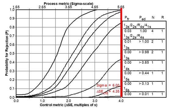
Figure 1. Power Function Graph showing “power curves” for a group of candidate QC procedures, as identified in the key at the right. Curves top to bottom match list of QC procedures top to bottom. For a 6-Sigma testing process, the medically important systematic error is shown by the vertical line at the far right (which is slightly off-scale on this graph).
Charts of Operating Specifications
These QC rejection characteristics can be incorporated in other tools, such as the Chart of Operating Specifications, or “OPSpecs Chart” [5-6] which is a more generic tool that is easier to use. The idea of an OPSpecs chart is to relate the quality goal (e.g., TEa requirement) to the operating specifications – the precision, bias, and QC that are necessary to assure a certain level of error detection, such as 90% Analytical Quality Assurance (AQA) for a stated allowable Total Error (TEa). Given a HbA1c quality requirement of 6.0%, Figure 2 shows the relationship between trueness (bias) on the y-axis and precision on the x-axis for the different QC procedures represented by the lines on the chart, which are identified in the key at the right side (where lines top to bottom correspond to rules and Ns top to bottom). To use this chart, an “operating point” is plotted where the y-coordinate represents the %bias observed for the method and the x-coordinate represents the %CV observed for the method. The lines to the right of the operating point represent QC rules that provide ≥ 90% error detection. The further to the right, the higher the error detection. On the other hand, the lines to the left of the operating point represent QC rules with ≤ 90% error detection - the further to the left, the lower the error detection.
For our example Method A, the operating has a y-coordinate of 0.0 and an x-coordinate of 1.0. Note the line immediately above the operating point represents the 1:3s N=1 rule, indicating at least 90% detection of medically important errors, confirming our earlier graphical assessment from the power curves. Note that the line for 1:6s N=1 (that corresponds to the metrologist’s recommended fixed limit) is far to the left of the operating point, indicating very low error detection.
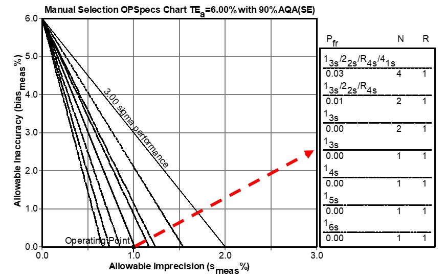
Figure 2. Chart of Operating Specifications for a Quality Requirement of 6.0%. An operating point is plotted to represent the method’s imprecision as the x-coordinate and the method’s bias as the y-coordinate. Any line above the operating point identifies a QC procedure that will provide appropriate error detection.
For another example, consider a HbA1c method that has a bias of 0.0% and a CV of 1.5%. Locate an operating point at x=1.5 and y=0.0, then observe that the only choice for this 4 Sigma method is a 1:3s/2:2s/R:4s/4:1s multirule procedure with N=4 when the objective is to achieve 90% detection of the medically important systematic error. Likewise, a method having a bias of 2.0% and a CV of 1.0% will also be a 4.0 Sigma method and would require the same multirule procedure with N=4. Again note that the line for 1:4s N=1 (corresponding to the recommended 6% fixed limit) is far to the left of the operating point so that QC procedure would provide very poor error detection.
Additional QC planning tools have been developed for selecting risk-based SQC strategies that identify the control rules, numbers of control measurements, and frequency of QC events. These include a Sigma-Metric Run Size Nomogram [7,8] and related calculators [9,10] that determine the frequency of QC in terms of the number of patient samples between QC events. These will be discussed later in this series.
What’s the point?
A general approach for assessing QC performance and selecting/planning appropriate QC procedures makes use of tools such as power function graphs or charts of operating specifications. These tools can readily assess the performance of fixed clinical acceptance limits on control charts. As illustrated here, rules such as 1:6s, 1:5s, and 1:4s, with N=1, offer very limited error detection, even for a high quality 6-sigma measurement procedure. Yet such applications would be entirely possible under the metrologists’ recommended re-design of IQC component I. With such poorly designed SQC strategies using clinical control limits, a laboratory’s only hope for detecting errors is “waiting for a miracle to come”.
The performance of fixed clinical limits can be readily predicted from SQC theory and is shown to be inadequate, as illustrated here. Thus, the metrologists’ recommendation to use fixed clinical control limits reveals a misunderstanding of how SQC procedures work, ignores the statistical theory for evaluating QC performance, and disregards an already established QC planning process that can be easily implemented with readily available QC planning tools [11]. The next part in this series will discuss the CLSI C24-Ed4 guidance for planning SQC strategies in more detail.
References
- Braga F, Pasqualetti S, Aloisio E, Panteghini M. The internal quality control in the traceability era. Clin Chem Lab Med 2021;59:291-300.
- Braga F, Panteghini M. Performance specifications for measurement uncertainty of common biochemical measurands according to Milan models. Clin Chem Lab Med 2021;59:1362-1368.
- Westgard JO, Quam EF, Barry PL. Establishing and evaluating QC acceptability criteria. Med Lab Observ 1994;26(2):22-26.
- Westgard JO, Groth T. Power functions for statistical control rules. Clin Chem 1979;25:863-9.
- Westgard JO, Hyltoft Petersen P, Wiebe DA. Laboratory process specifications for assuring quality in the U.S. National Cholesterol Education Program. Clin Chem 1991;37:656-61.
- Westgard JO. Charts of Operating Specifications (OPSpecs Charts) for assessing the precision, accuracy, and quality control needed to satisfy proficiency testing criteria. Clin Chem 1992;38:1226-33.
- Bayat H, Westgard SA, Westgard JO. Planning risk-based SQC strategies: Practical tools to support the new CLSI C24Ed4 guidance. J Appl Lab Med 2017;2:211-221.
- Westgard JO, Bayat H, Westgard SA. Planning risk-based SQC schedules for bracketed operation of continuous production analyzers. Clin Chem 2018;64:289-296.
- Westgard JO, Bayat H, Westgard SA. Planning SQC strategies and adapting QC frequency for patient risk. Clin Chim Acta 2021; 523:1-5.
- Westgard SA, Bayat H, Westgard JO. A multi-test planning model for risk based statistical quality control strategies. Clin Chim Acta 2021;523;216-233.
- CLSI C24-Ed4. Statistical Quality Control for Quantitative Measurement Procedures: Principles and Definitions – Fourth Edition. Clinical and Laboratory Standards Institute, 950 West Valley Road, Suite 2500, Wayne PA, 2016.