Basic Method Validation

The comparison of methods experiment is critical for assessing the systematic errors that occur with real patient specimens. Guidelines for performing the experiment are provided and there is an introductory discussion of how to graph the data and what statistics should be calculated.

• Purpose
• Factors to consider
  • Comparative method
  • Number of patient specimens
  • Single vs. duplicate measurements
  • Time Period
  • Specimen stability
• Data Analysis
  • Graph the data
  • Calculate appropriate statistics
• Criteria for acceptable performance
• Recommended minimum studies
• References

Purpose

A comparison of methods experiment is performed to estimate inaccuracy or systematic error. Review MV – The Experimental Plan to see how this experiment fits together with the other experiments. You perform this experiment by analyzing patient samples by the new method (test method) and a comparative method, then estimate the systematic errors on the basis of the differences observed between the methods. The systematic differences at critical medical decision concentrations are the errors of interest. However, information about the constant or proportional nature of the systematic error is also useful and often available from appropriate statistical calculations. Both the experimental design and the statistical calculations are critical for obtaining reliable estimates of systematic errors.

Factors to Consider

Comparative method

The analytical method that is used for comparison must be carefully selected because the interpretation of the experimental results will depend on the assumption that can be made about the correctness of results from the comparative method. When possible, a “reference method” should be chosen for the comparative method. This term has a specific meaning that infers a high quality method whose results are known to be correct through comparative studies with an accurate “definitive method” and/or through traceability of standard reference materials. Any differences between a test method and a reference method are assigned to the test method, i.e., the errors are attributed to the test method because the correctness of the reference method is well documented.

The term “comparative method” is a more general term and does not imply that the correctness of the method has been documented. Most routine laboratory methods fall into this latter category. Any differences between a test method and a routine method must be carefully interpreted. If the differences are small, then the two methods have the same relative accuracy. If the differences are large and medically unacceptable, then it is necessary to identify which method is inaccurate. Recovery and interference experiments can be employed to provide this additional information.

Number of patient specimens

A minimum of 40 different patient specimens should be tested by the two methods [1]. These specimens should be selected to cover the entire working range of the method and should represent the spectrum of diseases expected in routine application of the method. The actual number of specimens tested is less important than the quality of those specimens. Twenty specimens that are carefully selected on the basis of their observed concentrations will likely provide better information than the a hundred specimens that are randomly received by the laboratory. The quality of the experiment and the estimates of systematic errors will depend more on getting a wide range of test results than a large number of test results.

The main advantage of a large number is to identify individual patient samples whose results do not agree because of interferences in an individual sample matrix. This is often of interest when the new method makes use of a different chemical reaction or a difference principle of measurement. Large numbers of specimens – 100 to 200 – are recommended to assess whether the new method’s specificity is similar to that of the comparative method.

Single vs duplicate measurements

Common practice is to analyze each specimen singly by the test and comparative methods. However, there are advantages to making duplicate measurements whenever possible. Ideally, these duplicates should be two different samples (or cups) that are analyzed in different runs, or at least in different order (rather than back-to-back replicates on the same cup of sample). The duplicates provide a check on the validity of the measurements by the individual methods and help identify problems arising from sample mix-ups, transposition errors, and other mistakes. One or two such mistakes could have a major impact on the conclusions drawn from the experiment. At the least, such mistakes will cause much consternation in deciding whether or not discrepant results represent the performance of the method or whether they are “outliers” that should be removed from the data set. Duplicate analyses would demonstrate whether or not these observed discrepancies were repeatable.

If duplicates are not performed, then it is critical to inspect the comparison results at the time they are collected, identify those specimens where the differences are large, and repeat those analyses while the specimens are still available.

Time period

Several different analytical runs on different days should be included to minimize any systematic errors that might occur in a single run. A minimum of 5 days is recommended [1], but it may be preferable to extend the experiment for a longer period of time. Since the long-term replication study will likely extend for 20 days, the comparison study could cover a similar period of time and would require only 2 to 5 patient specimens per day.

Specimen stability

Specimens should generally be analyzed within two hours of each other by the test and comparative methods [1], unless the specimens are known to have shorter stability, e.g., ammonia, lactate. Stability may be improved for some tests by adding preservatives, separating the serum or plasma from the cells, refrigeration, or freezing. Specimen handling needs to be carefully defined and systematized prior to beginning the comparison of methods study. Otherwise, the differences observed may be due to variables in the handling of specimens, rather than the systematic analytical errors that are the purpose of the experiment.

Data analysis

Here’s where the going gets tough! There’s a lot of debate and discussion about the right way to analyze data from a comparison of methods experiment [2]. This has been going on for as long as I’ve been a clinical chemist and seems to be a chronic problem that flares up with each new generation of laboratory scientists. We studied the use and interpretation of statistics in method comparison studies almost twenty five years ago [3,4] and the lessons we learned still apply today. Our intention here is to provide some brief guidelines and then discuss the statistics in more detail later on in this series.

Graph the data

The most fundamental data analysis technique is to graph the comparison results and visually inspect the data. Ideally, this should be done at the time the data is collected in order to identify discrepant results that will complicate the data analysis. Any patient specimens with discrepant results between the test and comparative methods should be reanalyzed to confirm that the differences are real and not mistakes in recording the values or mixups of specimens.

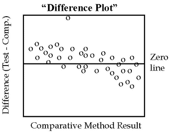
If the two methods are expected to show one-to-one agreement, this initial graph should be a “difference plot” that displays the difference between the test minus comparative results on the y-axis versus the comparative result on the x-axis, such as shown in the accompanying figure. These differences should scatter around the line of zero differences, half being above and half being below. Any large differences will stand out and draw attention to those specimens whose results need to be confirmed by repeat measurements.

Look for any outlying points that do not fall within the general pattern of the other data points. For example, there is one suspicious point in the plot shown here. Note also that the points tend to scatter above the line at low concentrations and below the line at high concentrations, suggesting there may be some constant and/or proportional systematic errors present.

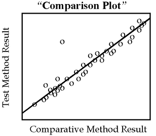
For methods that are not expected to show one-to-one agreement, for example enzyme analyses having different reaction conditions, the graph should be a “comparison plot” that displays the test result on the y-axis versus the comparison result on the x-axis, as shown by the second figure. As points are accumulated, a visual line of best fit should be drawn to show the general relationship between the methods and help identify discrepant results. Again, the purpose of this initial graphical inspection of data is to identify discrepant results in order to reanalyze specimens while they are fresh and still available.

However, this type of graph is generally advantageous for showing the analytical range of data, the linearity of response over the range, and the general relationship between methods as shown by the angle of the line and its intercept with the y-axis.

Calculate appropriate statistics

While difference and comparison graphs provide visual impressions of the analytic errors between the test and comparative methods, numerical estimates of these errors can be obtained from statistical calculations. Remember the inner, hidden, deeper, secret meaning of method validation is error analysis. You need to know what kinds of errors are present and how large they might be. The statistical calculations will put more exact numbers on your visual impressions of errors.

Given that the purpose of the comparison of methods experiment is to assess inaccuracy, the statistics that are calculated should provide information about the systematic error at medically important decision concentrations. In addition, it would be useful to know the constant or proportional nature of that error (review QC – The Experimental Plan for definitions of constant and proportional errors). This latter information is helpful in determining the cause or source of the systematic error and assessing the possibility of improving method performance.

For comparison results that cover a wide analytical range, e.g., glucose or cholesterol, linear regression statistics are preferable. These statistics allow estimation of the systematic error at more than one medical decision concentration to judge method acceptability and also provide information about the proportional or constant nature of the systematic error to assess possible sources of errors. Statistical programs typically provide linear regression or least squares analysis calculation for the slope (b) and y-intercept (a) of the line of best fit and the standard deviation of the points about that line (s_y/x). The systematic error (SE) at a given medical decision concentration (X_c) is then determined by calculating the corresponding Y-value (Y_c) from the regression line, then taking the difference between Y_c and X_c, as follows:

Y_c = A + bX_c
SE = Y_c - X_c

For example, given a cholesterol comparison study where the regression line is Y = 2.0 + 1.03X, i.e., the y-intercept is 2.0 mg/dL and the slope is 1.03, the Y value corresponding to a critical decision level of 200 would be 208 (Y = 2.0 + 1.03*200), which means there is a systematic error of 8 mg/dL (208 – 200) at a critical decision level of 200 mg/dL.

It is also common to calculate the correlation coefficient, r, which is mainly useful for assessing whether the range of data is wide enough to provide good estimates of the slope and intercept, rather than judging the acceptability of the method [3]. When r is 0.99 or larger, simple linear regression calculations should provide reliable estimates of the slope and intercept. If r is smaller than 0.99, it would be better to collect additional data to expand the concentration range, consider using t-test calculations to estimate the systematic error at the mean of the data, or utilize more complicated regression calculations that are appropriate for a narrower range of data [4].

For comparison results that cover a narrow analytical range, e.g., sodium or calcium, etc., it is usually best to calculate the average difference between results, which is the same as the difference between the averages by the two methods, also commonly called the “bias”. This calculated bias is typically available from statistical programs that provide “paired t-test” calculations. The calculations also include a “standard deviation of the differences” that describes the distribution of these between method differences and a “t-value” (t) that can be used to interpret whether the data are sufficient to conclude that there really is a bias or difference between the methods

For example, if the average of 40 analyses for sodium by the test method is 141.0 mmol/L and the average for the same specimens by the comparative method is 138.5, then the average systematic error, or bias, is 2.5 mmol/L (141.0 – 138.5). The algebraic sign of this bias is useful for showing which method is higher or lower, but it’s the absolute value of the difference that is important for judging the acceptability of the method.

Criteria for acceptable performance

The judgment of acceptability depends on what amount of analytical error is allowable without affecting or limiting the use and interpretation of individual test results [5]. This is complicated by the fact that any individual test result is also subject to random error, thus the overall or total error (TE) is composed of systematic error (SE) plus random error (RE). This “total error” can be calculated as follows:

TE_calc = SE + RE
TE_calc = bias_meas + 3s_meas

where smeas is the estimate of the method standard deviation from the replication experiment and biasmeas is the average difference or difference between averages from t-test calculations or the difference between Y_c-X_c where Y_c = a + bX_c from regression statistics. Method performance is acceptable when this calculated total error (TE_calc)is less than the allowable total error (TE_a). Remember that the CLIA proficiency testing criteria for acceptable performance are in the form of allowable total errors and provide a good starting point for setting analytical quality requirements.

Similar judgments on acceptability can be made using the graphical Method Decision Chart [6]. This chart allows you to plot bias_meas on the y-axis and s_meas on the x-axis, then judge acceptability by the location of this “operating point” relative to the lines for different total error criteria that are drawn on the chart.

Recommended minimum studies

Select 40 patient specimens to cover the full working range of the method. Analyze 8 specimens a day within 2 hours by the test and comparative methods. Graph the results immediately on a difference plot and inspect for discrepancies; reanalyze any specimens that give discrepant results to eliminate outliers and identify potential interferences. Continue the experiment for 5 days if no discrepant results are observed. Continue for another 5 days if discrepancies are observed during the first 5 days. Prepare a comparison plot of all the data to assess the range, outliers, and linearity. Calculate the correlation coefficient and if r is 0.99 or greater, calculate simple linear regression statistics and estimate the systematic error at medical decision concentrations. If r<0.99, estimate bias at the mean of the data from t-test statistics. Utilize the Medical Decision Chart to combine the estimates of systematic and random error and make a judgment on the total error observed for the method.

References:

1. NCCLS EP9-A: Method comparison and bias estimation using patient samples. National Committee for Clinical Laboratory Standards, Wayne, PA, 1995.
2. Hyltoft Petersen P, Stockl D, Blaaberg O, Pedersen B, Birkemose E, Thienpont L, Flensted Lassen J, Kjeldsen J. Graphical interpretation of analytical data from a comparison of a field method with a reference method by use of difference plots. Clin Chem 1997;43:2039-2046.
3. Westgard JO, Hunt MR. Use and interpretation of common statistical tests in method-comparison studies. Clin Chem 1973;19:49-57.
4. Cornbleet PJ, Gochman N. Incorrect least-squares regression coefficients in method-comparison studies. Clin Chem 1979;25:432-438.
5. Westgard JO, Carey RN, Wold S. Criteria for judging precision and accuracy in method development and evaluation. Clin Chem 1974;20:825-833.
6. Westgard JO. A method evaluation decision chart (MEDx chart) for judging method performance. Clin Lab Science 1995;8:277-283.