Sigma Metric Analysis
Multiple POC Glucose Methods
Sten Westgard, MS
In 2007, Scientists at the Mayo Clinic performed an interesting study of multiple POC glucose methods to evaluate their performance.We apply Westgard Sigma analysis to this data. Do you think world class performance is possible at the point of care?
- The Precision and Comparison data
- Calculate bias at the decision level
- Determine quality requirements at the critical decision level
- Calculate Sigma metrics
- Evaluation of performance by OPSpecs chart, Sigma-metrics graph, and EZ Rules 3
- Conclusion: what quality requirement to use?
January 2008
 |
[Note: This QC application is an extension of the lesson From Method Validation to Six Sigma: Translating Method Performance Claims into Sigma Metrics. This article assumes that you have read that lesson first, and that you are also familiar with the concepts of QC Design, Method Validation, and Six Sigma. If you aren't, follow the link provided.] |  |
More than ten years ago, we provided a QC application and analysis of a Point-of-care glucose method. With the debate over EQC and the CLIA Final Rules back on the front burner, we thought it would be interesting to "revisit" POC glucose methods and see what performance is being achieved by these devices.
The source of data for this QC application is a poster from the 2007 AACC conference: Evaluation of multiple point of care glucose methods compared to a laboratory hexokinase reference method, GR Deobald, LD Griesmann, RJ Scott, AM Wockenfus, BS Karon, Mayo Clinic, Rochester. This poster is, as of January 2007, in press for an article in Point of Care [Scott RJ, Deobald G, Griesmann L, Wockenfus AM, Karon BS. Evaluation of multiple point of care glucose methods compared to a laboratory hexokinase reference method. Point of Care, in press]
Dr Bradley Karon was gracious enough to provide additional precision data about this study.
Because of the results, we're going list some of the instruments anonymously. The reason will become clear.
The Precision and Comparison data
According to the abstract, 81 whole blood samples were analyzed by five different whole blood glucose methods and compared to results on the Roche Integra, which served as the reference method. In addition, Dr. Karon provided us with day-to-day precision estimates, obtained by using commercial control materials.
Imprecision Estimates:
| Method |
Low control
|
Medium Control
|
High Control
|
| Radiometer ABL 725 |
2.0%
|
2.0%
|
2.0%
|
| Method A |
6.0%
|
4.3%
|
2.7%
|
| Method B |
4.0%
|
2.3%
|
3.9%
|
| Method C |
4.3%
|
-
|
2.8%
|
| i-Stat |
1.4%
|
-
|
0.7%
|
There are a lot of different numbers to choose from. Do we evaluate all three levels? The best number? The worst number? Keep in mind that the CLIA quality requirement for glucose is a split requirement: Target value ± 6 mg/dL or ± 10% (whichever is greater). At low levels, the unit requirement kicks in, while any level above 60 mg/dL, the 10% requirement kicks in. What you pick to use here relies on your professional judgment
For the purposes of this QC application, we're going to use the medium control imprecision estimates - and take the average of the low and high control imprecision estimates for those methods that don't have a medium control. This means that the Inform will have a 3.6% and the i-Stat will have a 1.1% estimate imprecision.
Comparison of Methods Data:
Test Methods vs. Roche Integra 400 (N=81)
The range of glucose values for this study was 36 - 410 mg/dL, with a median glucose value of 120 mg/dL.
| Method |
Slope
|
y-intercept
|
r
|
| Radiometer ABL 725 |
1.03
|
-1
|
0.995
|
| Method A |
0.97
|
4
|
0.981
|
| Method B |
0.99
|
12
|
0.977
|
| Method C |
0.92
|
6
|
0.984
|
| i-Stat |
0.97
|
-2
|
0.998
|
Remember that the correlation coefficient is not the key statistic here. The value of the correlation coefficient merely tells us that simple linear regression would be sufficient for these analytes (for those r values below 0.95, other forms of regression like Deming or Passing-Bablock are preferable, but in this case, are not available).
Calculate bias at the decision level
Now we take the comparison of methods data and set the equation to the level covered in the imprecision study. We're going to the 120 mg/dL median level as the decision level of interest. Using that level, we can solve the equations and obtain bias estimates.
Here are the steps for calculating bias:
((slope*level) + YIntercept) - level) / level = % bias
Here is an example calculation for the ABL 725:
((1.03*120.0) -1) - 120.0) / 120.0 = ((123.6 - 1) - 120.0) / 120.0
(122.6 - 120.0) / 120.0 = 2.6 / 120.0 = 0.02166 * 100 = 2.2%
| Method |
Slope
|
y-intercept
|
Bias%
|
| Radiometer ABL 725 |
1.03
|
-1
|
2.2%
|
| Method A |
0.97
|
4
|
0.3%
|
| Method B |
0.99
|
12
|
9.0%
|
| Method C |
0.92
|
6
|
3.0%
|
| i-Stat |
0.97
|
-2
|
4.7%
|
Determine the quality requirements at the critical decision level
Now that we have both bias and CV estimates, we are almost ready to calculate the Sigma metrics for these analytes. The last (but not least) thing we need is the quality requirement for the method. As we mentioned earlier, CLIA provides a split quality requirement, Target value ± 6 mg/dL or ± 10% (greater). Given the reference median method level of 120 mg/dL, the appropriate analytical quality requirement for a laboratory method is 10%.
BUT, we are dealing with point-of-care devices, where the quality requirements are confusing and different. When these (often CLIA-waived) glucose devices are used at home or non-laboratory settings, the most commonly-stated quality requirement for a non-laboratory method is an error grid with essentially 20% allowable error. For example, at a level of 120 mg/dL, the acceptable error is up to 24 mg/dL (i.e. a value of 96 mg/dL and 120 mg/dL may not be different values).
Calculate Sigma metrics
Now we have all the pieces in place.
Remember the equation for Sigma metric is (TEa - bias) / CV:
For the Radiometer ABL 725 metric is (20.0 - 2.2) / 2.0 = 8.9
| Source |
CV%
|
Bias%
|
Sigma metric
for 20% |
Sigma metric
for 10% |
| Radiometer ABL 725 |
2.0%
|
2.2%
|
8.9
|
3.9
|
| Method A |
4.3%
|
0.3%
|
4.58
|
2.26
|
| Method B |
2.3%
|
9.0%
|
4.78
|
0.43
|
| Method C |
3.6%
|
3.0%
|
4.72
|
1.94
|
| i-Stat |
1.1%
|
4.7%
|
13.9
|
4.82
|
Given the relaxed requirement of 20%, most of these methods perform admirably and a few provide world class performance. If we apply the laboratory standard, however, three methods are below the 3.0 Sigma threshhold - in industry terms, those methods would not be considered acceptable for routine production or operation.
Both the Radiometer ABL 725 and the i-Stat provide good performance at the laboratory standard and world class performance for the "home use" standard. Again, your professional judgment is needed to determine what standard is most appropriate.
Evaluation of Performance by OPSpecs chart, Sigma-metrics graph, and EZ Rules 3
Using EZ Rules 3, you can determine the optimum QC Design for each of these methods. By using Automatic QC Selection, you can see the ideal rules and controls needed to provide appropriate QC.
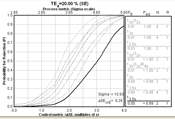
Here's the Sigma-metrics chart for the 20% requirement. The optimal QC procedure is 3 controls with 3.5s limits. (Actually, the program "maxes out" at 3.5s limits, so it's even possible that wider limits would be possible!).
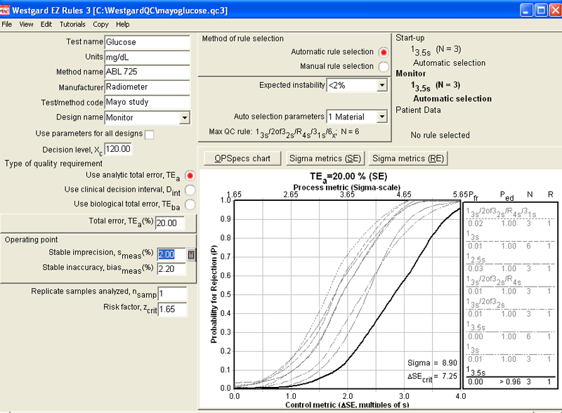
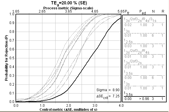
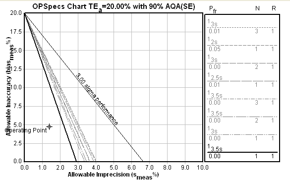
Here's a close-up of the Sigma-metrics chart (below), which shows that the ABL 725 will detect essentially all critical errors within the first run, while suffering from essentially no false rejection.
Here is the OPSpecs chart for the ABL 725 (below):
For the i-Stat, the Sigma-metrics chart looks about the same. The i-Stat is set up to use just two controls instead of three, but its method performance means that the reduction in controls does not require an increase in needed QC. The choice of 3.5s limits and two controls provides, as with the ABL, great error detection and essentially no false rejection.
Conclusion: What method would you choose? What QC would you perform?
Ironically, many of the methods studied in this paper are waived methods. That is, you don't have to do any extra QC beyond the manufacturer recommendations. As long as you follow manufacturer instructions, you don't actually have to monitor QC performance in this manner or make any changes to the QC you implement.
For the purposes of this application, however, we're going to assess the QC required by the methods, regardless of their regulatory classification. After evaluation with EZ Rules 3, here is the summary of QC recommendations:
| Source |
CV%
|
Bias%
|
Recommended QC for 20%
|
Pfr
|
| Radiometer ABL 725 |
2.0%
|
2.2%
|
13.5s with N=3
|
0
|
| Method A |
4.3%
|
0.3%
|
12.5s with N=3
|
3%
|
| Method B |
2.3%
|
9.0%
|
12.5s with N=3
|
3%
|
| Method C |
3.6%
|
3.0%
|
12.5s with N=2
|
3%
|
| i-Stat |
1.1%
|
4.7%
|
13.5s with N=2
|
0
|
Given the less-demanding quality requirement of 20%, all of these methods can use wider limits than the usual 2s limits. Looking at the last column, you see that false rejection for these methods is acceptable (the goal is to be less than 5%). When QC is implemented with "traditional" 2s control limits and Ns of 2 or 3, the false rejection rates are normally between 9% and 14%. The world class methods have basically eliminated that false rejection problem, while the other methods have reduced false rejection to a third or a fifth of the usual rate.
Now let's assess all these methods against the laboratory standard. Again, we use EZ Rules 3 to evaluate performance and obtain the best QC recommendations. This time, however, we find that the news here isn't quite as rosy:
| Source |
CV%
|
Bias%
|
Recommended QC for 10%
|
Ped
|
| Radiometer ABL 725 |
2.0%
|
2.2%
|
12.5s with N=3
|
72%
|
| Method A |
4.3%
|
0.3%
|
MAX QC: 13s/2of32s/R4s/31s/6x with N=6
|
23%
|
| Method B |
2.3%
|
9.0%
|
MAX QC: 13s/2of32s/R4s/31s/6x with N=6
|
0
|
| Method C |
3.6%
|
3.0%
|
MAX QC: 13s/22s/R4s/31s/8x with N=4
|
5%
|
| i-Stat |
1.1%
|
4.7%
|
13s with N=2
|
93%
|
Note that for our three anonymous methods, even using full "Westgard Rules" does not provide enough QC power to detect medically important errors. There is simply too much random (CV) and systematic (bias) errors for these methods to satisfy the laboratory standard of performance.
The Radiometer ABL and the i-Stat, in contrast, have workable QC recommendations and the desired level of error detection. They are meeting the laboratory standard of performance.